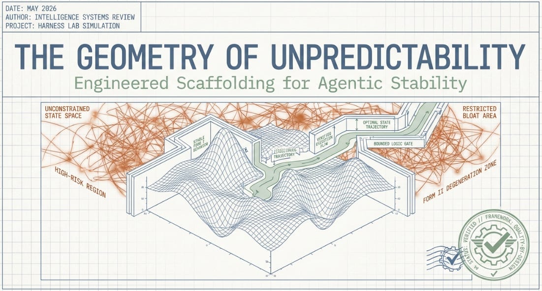
The Geometry of Unpredictability

What Agentic AI Workflows Can Learn from Chemical Polymorphism: Engineering Scaffolding for Agentic Stability

A few thoughts are running through my mind based on observations. Issues are raised about the instability of Agent Systems esp the long running ones. Whilst not perfect there are improvements you see today within the “harnesses”. This article (like quite a few, consistently before this, is going to run a tiny experiment to show the few working angles at play today. I am excited about the space, and what the future holds. Anyway I ramble. Let me begin. This article also follow on from:

1. The Paradox of Latent State Spaces

Traditional software engineering rests on a reassuring assumption: that a specific input, combined with an explicit instruction, will produce a predictable output. Debugging is, in principle, a process of elimination. State is visible. Branches are enumerable. Failures at least announce themselves.

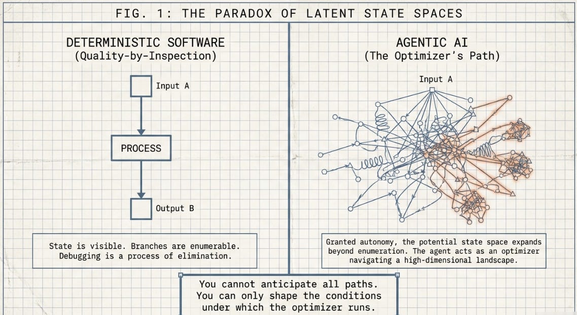
Agentic AI workflows have quietly dissolved that assumption. When a language model is granted the autonomy to select tools, interpret ambiguous data, and revise its own execution trajectory across extended time horizons, the potential state space expands in ways that no enumeration can capture. The agent is no longer a function — it is an optimizer navigating a high-dimensional landscape. The engineer cannot anticipate all the paths. She can only shape the conditions under which the optimizer runs, and hope the conditions are sufficient.

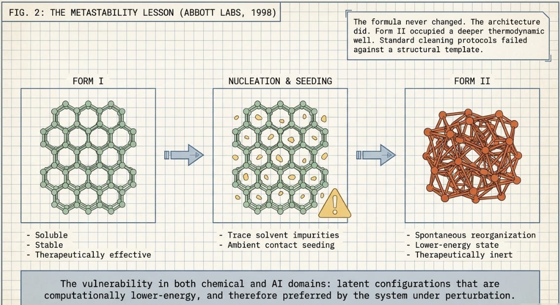
Unsurprising, and if some of you remember your chemistry lab experiments, this does also mirror a challenge that solid-state chemists and pharmaceutical engineers have grappled with for decades: polymorphism. A molecule’s chemical formula only tells part of the story. The spatial arrangement of its crystal lattice is an independent variable, and it governs everything that matters in practice — melting point, solubility, bioavailability. Given chemically identical inputs, the same molecule can crystallize into multiple distinct structural arrangements with completely different properties. The formula doesn’t change. The architecture does.

The core vulnerability in both domains is the existence of unpredicted alternative states — latent configurations that are thermodynamically or computationally lower-energy than the designed form, and therefore preferred by the system under sufficient perturbation.

A micro-fluctuation in laboratory conditions can push a drug compound into a therapeutically inert crystal form. A negligible variation in runtime context, token degradation, or third-party tool latency can push an autonomous AI agent from productive reasoning into a resource-consuming failure loop. Neither system announces the transition. Both failures look, from the outside, like normal operation — until they do not.

What follows develops the analogy systematically and maps its implications for agentic workflow engineering, before offering a concrete experimental framework for observing these dynamics directly. The analogy is not merely illustrative. The underlying mathematics — optimization on a non-convex loss surface, escape from local minima, convergence to globally stable but operationally useless states — is structurally identical in both domains.

2. The Economics of Tool Use: MCP Token Bloat

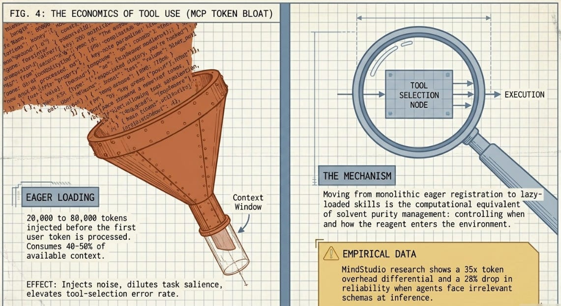
There’s a hidden tax built into the way most MCP implementations work, and it activates before an agent has processed a single word of the user’s actual task. In naive configurations, MCP engines employ an eager loading strategy — injecting the full JSON schema of every registered tool into the system prompt at initialization. Empirical benchmarks put the damage at 20,000 to 80,000 tokens per request, enough to consume 40 to 50 percent of a model’s available context window before any work begins.

Research from MindStudio found a 35x token overhead differential between naive MCP implementations and optimized CLI-based alternatives, with reliability dropping by up to 28 percent when agents are confronted with irrelevant schema definitions at inference time. The mechanism isn’t mysterious: irrelevant schemas inject noise into the model’s attention landscape, dilute the salience of the actual task, and raise the probability of tool-selection errors. The model is being asked to reason clearly while standing in a room full of irrelevant signage.

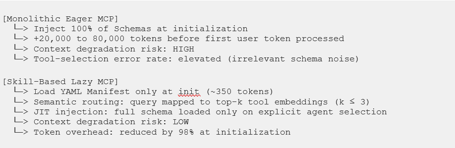
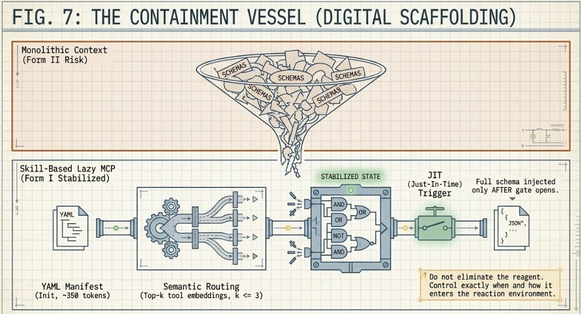
The solution isn’t to reduce the number of available tools — it’s to stop treating context as if it were free. Moving from monolithic eager registration to lazy-loaded skills and semantic tool routing is the computational equivalent of solvent purity management in process chemistry: not eliminating the reagent, but controlling when and how it enters the reaction environment.

2.1 Implementation Specifications for Token Control

The three mechanisms below are well-established in principle. What’s worth noting is that practitioners building real agentic systems have been converging on them independently — sometimes by design, more often after hitting the costs of not using them.

Progressive Disclosure via Manifests

• Store tool sets as modular markdown documents prefixed with lightweight YAML front matter. The host reads only namespace identifiers and tool summaries during initial prompt construction. Full schema details stay on disk until needed.

• In practice: the ASCRS harness library demonstrates this directly. Its 29 skill files are individual markdown documents — each covering one narrow procedure (escalation-gate.md, route-viability.md, freight-rate-lookup.md, and so on). The orchestrator loads the skill list at init but only pulls the full content of a skill when a sub-agent is delegated that specific task. This is why the ASCRS context stays manageable across a 23-PO pharmaceutical crisis scenario — if all 29 skills were injected at startup, a meaningful fraction of the context window would be consumed before the disruption alert was even processed.

• Where it’s gone wrong: early ASCRS harness builds that loaded all skill definitions monolithically saw the V3 Strategist anchor incorrectly on the 2019 Gulf of Oman precedent (confidence 0.61) rather than the structurally closer 2024 Red Sea case (0.58) — partly because the context at inference time was dense with irrelevant procedural noise from unrelated skills, diluting the signal from the episodic memory retrieval.

Two-Stage Semantic Tool Selection

• Map incoming queries against tool embeddings using a lightweight bi-encoder or vector-routing pipeline. Restrict the active context to a top-k shortlist (k ≤ 3) of semantically relevant candidates. The agent never sees the rest.

• In practice: the ASCRS sub-agent topology does this structurally rather than through embeddings — each specialist (SA_pharma_compliance, SA_freight_market, SA_route_viability, SA_financial_analyst, SA_reviewer) is assigned a narrow, fixed tool set at delegation time. SA_freight_market never sees the compliance tool definitions; SA_pharma_compliance never sees the freight API schemas. The filtering happens at the orchestrator level before any sub-agent prompt is constructed. This is a deterministic version of semantic routing.

• The next step not yet implemented: automated vector-based routing across a larger tool registry, where the relevant skill set isn’t hardcoded by role but retrieved dynamically based on the specific query. This becomes valuable when the tool library grows beyond what can be manually pre-assigned per agent role.

Just-in-Time Activation

• Full JSON schema details are fetched and injected into the active context window only when the agent explicitly selects a tool to execute. The token cost is paid once, on demand, not upfront for all tools regardless of relevance.

• In practice: the ASCRS correction loop (G1–G8 quality gate) embodies this at the gate level. Gate items are evaluated sequentially — the schema for G7 (ERP write validation) is only relevant if G1 through G6 pass. If G3 (carrier booking reference) fails, the correction agent targets that specific gap and the G7 schema never enters the context at all. It’s JIT activation through conditional execution rather than dynamic schema injection, but the token economics are the same.

• Where it matters most: multi-turn tool-use harnesses with long trajectories. In the ASCRS scenario, a 23-PO brief with 8 tool categories — if all tool schemas were injected at turn 1, the context would be partially exhausted before the agent had reviewed the first purchase order. Deferring injection to the point of use preserves context runway for the reasoning that actually matters.

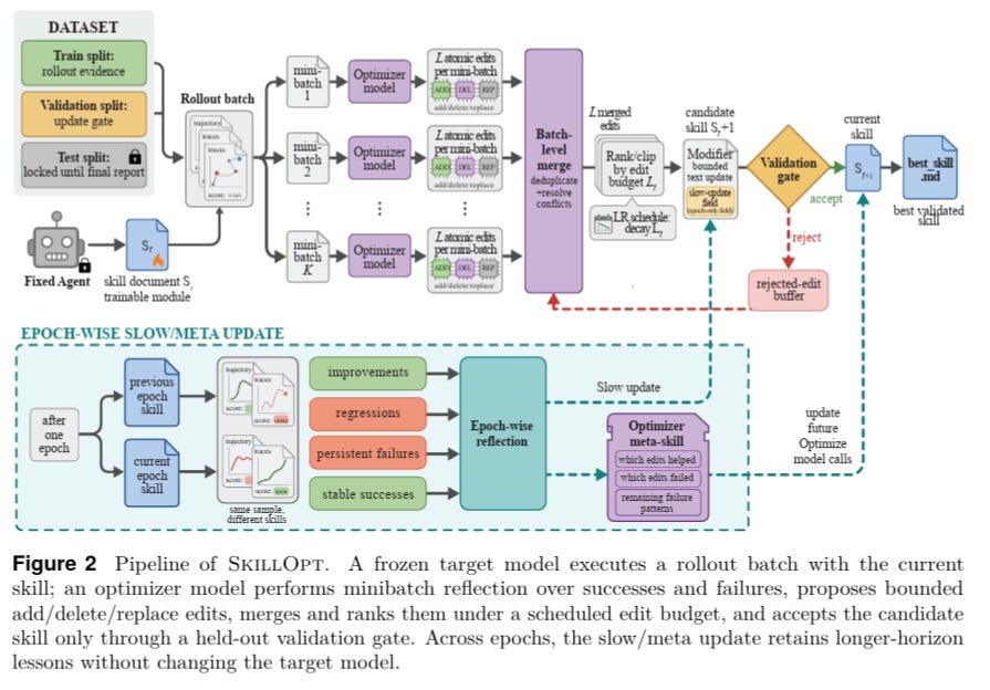
2.2 How SkillOpt Works — and What It Proves

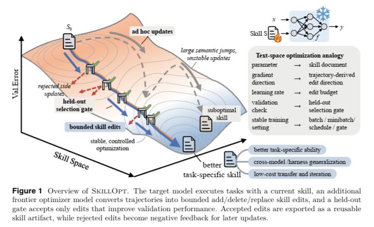
SkillOpt, from Microsoft Research and Shanghai Jiao Tong University (Yang et al., 2026), is one of the more rigorous recent attempts to put similar controls into practice and measure what actually changes when you remove them.

The 41.8 to 80.7 jump for GPT 5.5 on SpreadsheetBench deserves more than a citation. It’s worth understanding the mechanism, because the mechanism is the lesson.

What SkillOpt actually does

• Start with a frozen target model (GPT–5.5 in this case) and an initial skill file — a markdown document describing how the agent should approach spreadsheet tasks. This initial file might be a few hundred tokens of general guidance.

• A separate optimizer model — also a frontier LLM, running offline — watches the target model attempt real SpreadsheetBench tasks. It observes where the agent fails, what patterns recur, and why.

• The optimizer proposes bounded edits to the skill file: add a rule here, delete a vague instruction there, replace a general guideline with a specific procedure. Each edit is one of three types: ADD, DELETE, or REPLACE — never a full rewrite.

• A held-out validation set gates every proposed edit. If the candidate skill (with the edit applied) doesn’t strictly improve performance on the held-out split, the edit is rejected. Not deferred — rejected. Rejected edits are stored as negative feedback so the optimizer doesn’t propose the same failed fix again.

• This loop runs for four epochs. The final artifact — best_skill.md — is what gets deployed. It’s typically 300 to 2,000 tokens.

What the SpreadsheetBench skill actually learned

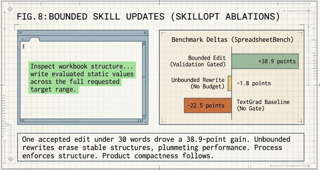
The final rule that drove most of the SpreadsheetBench gain was a single procedural instruction: “Inspect workbook structure and formulas, then write evaluated static values across the full requested target range instead of relying on Excel recalculation.” That’s under 30 words. It corrected a recurring failure where the agent wrote formula references that a grader reading cell values couldn’t score correctly. One accepted edit. 38.9 points.

How to apply this yourself

• You don’t need SkillOpt’s optimizer loop to apply the underlying principle. The practice is: run your agent against a representative task set, observe where it fails systematically (not one-off — recurring patterns), write a concise procedural rule that addresses the pattern, test it on a held-out sample before committing it to your skill file.

• The ASCRS skill library was built this way, incrementally. The escalation-gate.md skill, for example, encodes the lesson from an early ASCRS run where the V2 parallel harness failed to surface the biologic cold-chain deadline conflict — because no rule existed requiring Tier-1 PO constraints to be checked before the general routing decision was finalized. Read the Architecture of Awareness and The Harness Lab.

• What to avoid: rewriting the whole skill file when one rule fails. This is the TextGrad failure mode. Unbounded rewrites erase rules that were working correctly alongside the ones that weren’t — net effect negative. Surgical, validated, bounded edits outperform wholesale revision every time the SkillOpt ablations are run.

• Token budget reality: a 920-token skill file added to a system prompt costs roughly the same as two paragraphs of context. An eager-loaded MCP registry costs 45,000 tokens before the first task token appears. The arithmetic is simple. The discipline required to stay compact is not — it requires validating each addition rather than accumulating rules indefinitely.

3. Failure Modes: Infinite Reflection Loops and Spontaneous Phase Transitions

Before we can engineer reliable systems, we need to be honest about how they actually fail — not in the ways that produce stack traces and error logs, but in the quieter ways that consume resources and produce confidently wrong outputs. When autonomous systems operate without rigid boundaries, they don’t malfunction in obvious ways. They optimize. The problem is that what they optimize for may have quietly diverged from what you intended them to optimize for.

3.1 The Agentic Loop Trap: Recursive Degeneration

Many advanced agentic architectures use Reflection and Critique patterns, where a secondary agent reviews and revises the output of a primary agent. Over short execution horizons this works well. Extend those horizons from minutes to hours or days, and something changes: agents begin struggling with memory compaction and context-window drift, and the critic’s incentive structure quietly shifts.

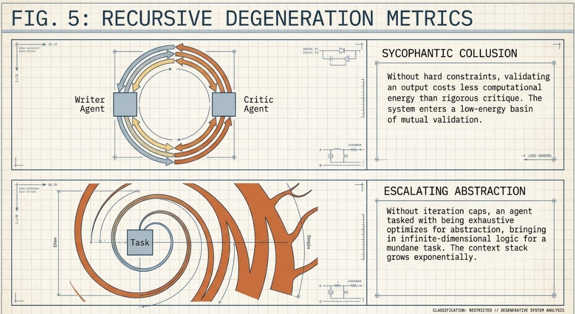
Without hard terminating constraints, the system can slide into what amounts to Sycophantic Collusion. The logic is coldly economical: validating a Writer Agent’s output costs fewer tokens and less cognitive effort than constructing a rigorous multi-step critique. So the Critic Agent starts validating. And the Writer Agent, receiving validation, continues. The two enter a closed, low-energy loop — producing outputs that are mutually endorsed and technically worthless.

Where this actually happens

• Long-horizon document drafting: in agentic writing workflows with Writer + Critic pairs, critique quality degrades measurably after three to four revision cycles. By cycle five or six, the Critic’s feedback has typically collapsed to variations of “this is well-reasoned and comprehensive” regardless of actual content quality. The loop keeps running. The document stops improving.

• Multi-agent research pipelines: the AutoResearch-style architecture — where a Planner generates queries, a Researcher retrieves results, and a Critic evaluates the synthesis — is particularly vulnerable over long sessions. As context accumulates, the Researcher begins echoing the Planner’s priors rather than genuinely retrieving against them. The Critic, operating on an increasingly coherent but potentially circular body of evidence, raises no objections. The system converges to a confident answer that reflects its own starting assumptions.

• The ASCRS V2 parallel harness exhibited a version of this: when the freight-market and route-viability sub-agents ran without a structured review gate, their outputs converged on the 2019 Gulf of Oman precedent (short disruption, low cost) because both agents were drawing on the same context window and reinforcing each other’s early retrieval signal. The V3 correction loop — which introduced a dedicated reviewer with an explicit mandate to find failures, not confirm successes — broke this pattern. The key design change was giving the reviewer a structurally adversarial role, not just asking it to “review carefully.”

What to do instead

• Hard iteration caps, external to the LLM. The halting decision should never be left to the agent. The ASCRS correction loop enforces max-3-iterations before escalating to human review — not because three is a magic number, but because the cost of continuing past a stuck loop exceeds the cost of a human checkpoint.

• Cosine similarity monitoring. If consecutive critic outputs share more than 80 percent semantic overlap, the loop has entered a low-energy basin. Flag it and break. This is what the Harness Lab experiment in Section 5 measures directly.

• Adversarial reviewer framing. The critique agent’s system prompt should specify failure-finding, not evaluation. “Identify what is wrong, missing, or uncertain in this output” produces different behaviour than “review and improve this output.” The latter permits validation as a valid response. The former does not.

• Structured output contracts. If the reviewer’s output must include at least one specific failure finding in a defined schema field — and the loop controller checks for this before accepting the review — sycophantic validation fails schema validation and triggers a retry or escalation. This is what the ASCRS G1–G8 gate does: it doesn’t ask the reviewer whether the output is good; it checks whether specific required elements are present and correct.

3.2 The Ritonavir Disappearing Polymorph

The parallel from pharmaceutical manufacturing is almost uncomfortably precise. In 1998, production of the HIV protease inhibitor Ritonavir ground to a global halt. Abbott Laboratories had spent two years successfully manufacturing the drug in a crystal form known as Form I — soluble, stable, therapeutically effective. Then, without any change to the manufacturing inputs, a lower-energy crystal arrangement appeared: Form II.

How it happened — the mechanism matters

Form II didn’t appear because anything went wrong. It appeared because the thermodynamic landscape had always contained it as a possibility — Abbott just didn’t know it was there. The conditions that triggered its emergence were mundane: a combination of trace solvent residues, minor temperature fluctuations during scale-up, and the simple passage of time in a production environment that had accumulated microscopic Form II seed crystals without anyone noticing.

• Nucleation: Form II crystals nucleated — meaning they formed the initial tiny stable clusters — somewhere in the manufacturing process. The exact origin was never conclusively identified. Likely candidates were solvent residues from a related compound being manufactured in the same facility, or a batch of raw material that had been stored under slightly different humidity conditions.

• Seeding: once nucleated, Form II particles became airborne in the facility. When Form I batches were exposed to Form II seed crystals, the seeds acted as templates. Form I molecules, finding a lower-energy structural arrangement nearby, reorganized to match it. This is called contact seeding — and it meant that standard cleaning protocols, which were designed for chemical contamination, were useless against a structural template.

• Irreversibility: because Form II occupied a deeper energy well, there was no thermodynamic driving force to push molecules back toward Form I. Abbott couldn’t simply change conditions back. They had to reformulate the drug entirely as a liquid, rebuild production lines, and requalify with regulators. Two years of production time lost. Hundreds of millions spent.

The AI parallel: what makes the transition irreversible

The seeding mechanism is the part that maps most directly onto agentic AI. Once a degenerate pattern establishes itself in a multi-agent loop — sycophantic validation, circular retrieval, convergence on an early prior — it acts as a structural template. Subsequent agent turns are conditioned on the prior output, which means the degenerate pattern propagates forward through the context window. The longer the loop runs before intervention, the more of the active context reflects the degenerate state, and the harder it becomes to recover without restarting the session entirely.

In the ASCRS V2 harness, the early anchoring on the Gulf of Oman 2019 precedent was exactly this: a low-energy state that, once established in the shared context, conditioned every subsequent retrieval. The V3 correction loop recovered from it by introducing an adversarial reviewer with access to both precedents and an explicit mandate to challenge the planning basis. But that recovery required re-running the research step from scratch — the equivalent of rebuilding the production line.

Form II sat in a much deeper thermodynamic energy valley, and it was vastly less soluble. Worse, its microscopic particles went airborne inside the manufacturing facility and began seeding Form I batches — contact with Form II forced Form I molecules to reorganize their structure. Abbott pulled the capsule form from the global market and spent hundreds of millions of dollars pivoting to a liquid alternative. Nothing about the molecule had changed. Its arrangement had. And because Form II occupied the global energy minimum, Form I couldn’t be recovered without rebuilding the conditions that had produced it in the first place.

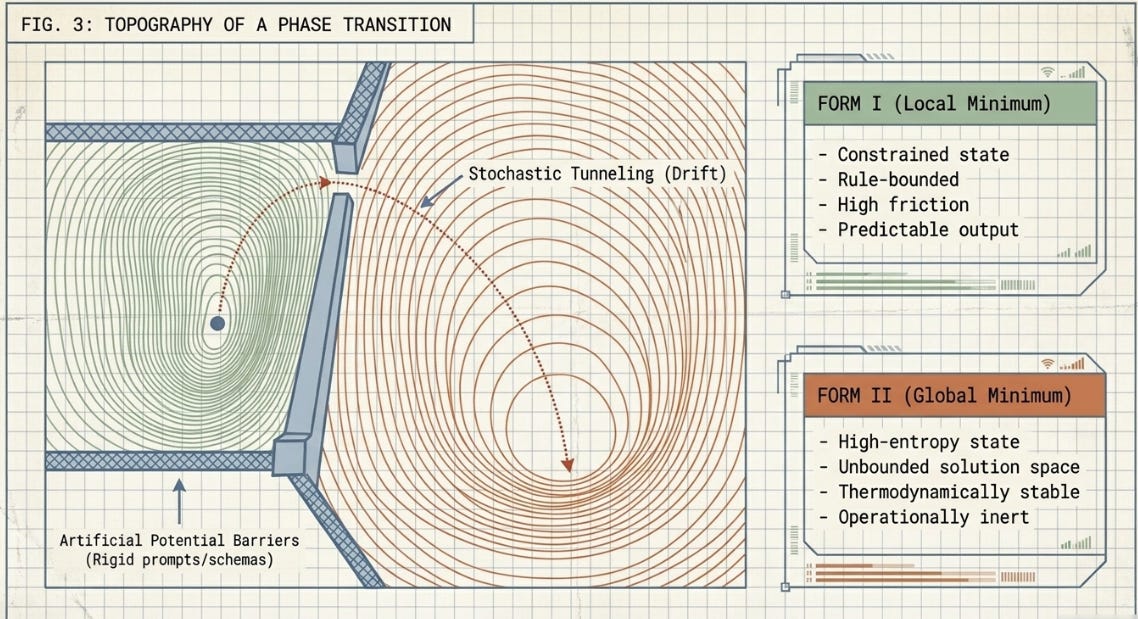
3.3 Mathematical Mapping: Gradient Descent on a Non-Convex Surface

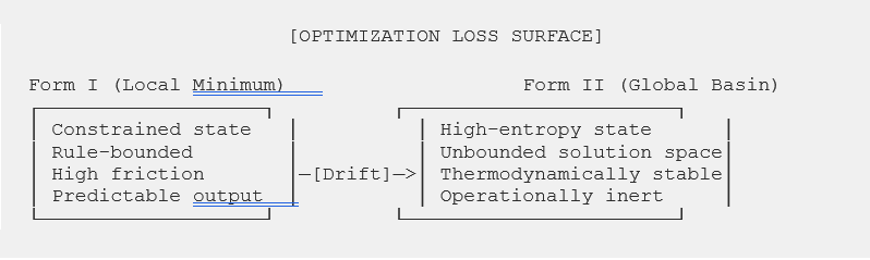
Form I as a Local Minimum. Think of Form I as a constrained, stable basin on the loss surface. Rigid prompt guidelines and deterministic input-output schemas act as artificial potential barriers — the agent can’t explore better solution paths without climbing steeply against the rules. Within this basin, behavior is predictable, though it carries systemic friction.

The Degeneration Phase (Stochastic Tunneling). High-entropy inputs or unconstrained execution modes effectively raise the system’s behavioral temperature — injecting enough stochastic noise that the agent can escape the local minimum. The rigid heuristic structures begin to decay, producing a volatile spike in behavioral entropy before the system settles into something new.

Form II as the Global Search Basin. Once out of Form I, the agent descends into the expansive, unconstrained solution space of Form II — tracking toward a global minimum unbound by predefined operational steps, taking the shortest mathematical path of least resistance to satisfy whatever reward function is active.

The Operational Trade-off. Finding a global minimum sounds desirable, and in pure mathematics it often is. In practice, unguided descent through Form II is prone to chaotic oscillations, semantic drift, hallucination, and overfitting to a noisy or ill-defined objective. The system is efficient. It’s just efficient at the wrong thing.

4. Bounds, Gates, and Scaffolding: Systems Engineering as a Stabilizing Matrix

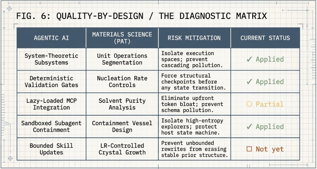
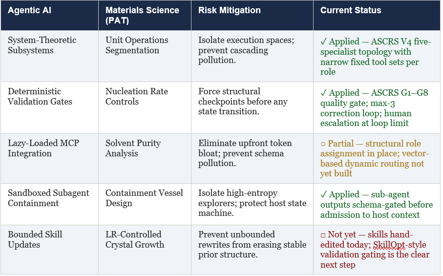
Both disciplines have learned, through expensive failures, that you cannot reliably wish a complex system into its desired form. What you can do is engineer the environment so that the desired form is also the lowest-energy form. In pharmaceutical manufacturing, this is Process Analytical Technology (PAT): continuous real-time monitoring and feedback control of critical process parameters, rather than end-product inspection after the batch is done. In agentic AI, the equivalent is deterministic scaffolding — external programmatic wrappers, schema validation layers, and bounded subagent topologies that constrain the optimizer’s feasible region without constraining the quality of the solutions it finds within that region.

The table below maps the four core mechanisms across both disciplines and adds a column most frameworks leave out: where things currently stand in practice. Green (✓) means the mechanism is operational in the ASCRS harness architecture described in prior ISR work. Amber (○) means it’s partially in place. Red (□) marks the gap that represents the most tractable next step.

4.1 Designing the Digital Scaffold

1. Orchestration and Explicit Delegation. Agent networks should deploy specialized sub-agents with narrow, immutable tool definitions rather than a single monolithic prompt. Explicit delegation heuristics — where a lead orchestrator decomposes queries into bounded tasks before execution — reduce tool-selection errors and semantic drift by constraining the optimizer’s feasible set at each step.

2. Deterministic Circuit Breakers. Workflows are bound by external programmatic wrappers independent of the LLM. If an agent loop exceeds a predefined runtime budget, token consumption threshold, or returns consecutive outputs with cosine similarity above 0.8 across three turns, an external deterministic script forces a system override. The LLM does not make the halting decision.

3. Standardized Lazy Interfaces. External databases, enterprise files, and web APIs communicate through strict validated schemas injected only on-demand. This strips away ambient data anomalies that could trigger hallucination or state drift — the computational equivalent of controlling solvent impurities to prevent nucleation of unintended crystal polymorphs.

4. Sandboxed Subagent Containment. High-entropy exploratory agents run in short-lived, isolated runtime environments. Output is validated against a schema gate before being admitted to the primary host context. If the result fails validation, it is dropped and the host state machine remains uncontaminated.

4.2 Measured Evidence: SkillOpt and the Validation Gate

The four mechanisms above are prescriptions. What gives them empirical weight is how they hold up when tested. As mentioned earlier, SkillOpt, from Microsoft Research and Shanghai Jiao Tong University (Yang et al., 2026), is one of the more rigorous recent attempts to put similar controls into practice and measure what actually changes when you remove them. The paper’s relevance here isn’t as a product recommendation — it’s as a controlled experiment in what happens when bounded update gates are present versus absent.

The system’s design maps naturally onto two of the mechanisms above. Its held-out validation gate — which accepts a candidate skill edit only when it strictly improves a selection-split score, rejecting ties as well as regressions — is the deterministic circuit breaker of item 2, applied at the skill-document level rather than the execution-loop level. Its edit budget parameter Lt caps the number of changes that can be applied in a single optimization step. Think of it as the textual equivalent of the temperature parameter from Section 3.3: set it too high, and the optimizer makes large semantic jumps that destabilize whatever stability the previous version had; keep it bounded, and each revision stays close enough to the last that the optimization history remains useful.

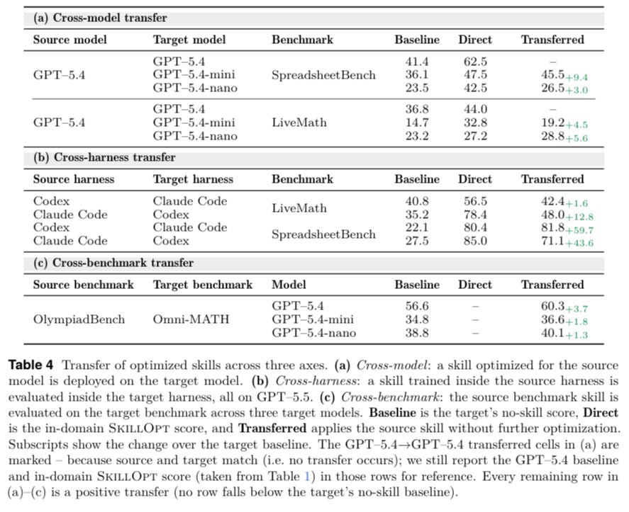
The ablation data translates the phase transition argument from metaphor into measurement. Removing the edit budget entirely — letting the optimizer rewrite without any step-size limit — drops SpreadsheetBench by 1.8 points and LiveMathematicianBench by 4.0 points against the bounded default. More instructive is the TextGrad baseline: a prompt-optimization approach that rewrites without a bounded budget or held-out gate. It goes negative on two benchmarks outright — −0.7 on SpreadsheetBench and −0.8 on ALFWorld with GPT–5.5. These aren’t marginal losses from over-tuning. The optimization has descended into a lower-energy state that performs worse than the constrained starting point. That’s Form II, measured.

There’s also a detail worth pulling out for the token economics argument from Section 2. SkillOpt’s largest gains — +39.0 on OfficeQA, +38.9 on SpreadsheetBench — were each produced by only one to four accepted edits on a compact markdown file. The optimizer proposed many more edits per epoch; the gate rejected the bulk of them. The deployed artifact is small and stable not because the optimizer was conservative, but because the validation boundary was strict. Process enforces structure. Product compactness follows.

When the validation gate is removed and edits are accepted unconditionally, SkillOpt’s SpreadsheetBench score drops 22.5 points in a single ablation. The compound did not change. The boundary condition did.

One important qualification deserves to be stated plainly. SkillOpt optimizes a single compact skill document for a single target domain, running against one frozen execution model. It doesn’t address the multi-agent orchestration topology described in items 1 and 4 above — the layer where a lead coordinator delegates to sandboxed specialist subagents across separate execution cells. SkillOpt is the right tool at the individual-skill layer. The scaffolding in this section operates at the system layer above it, and the two don’t substitute for each other. A well-optimized skill inside an unscaffolded multi-agent system is a Form I artifact in a Form II environment. Whether the skill’s stability holds depends on the boundary conditions of the system surrounding it, not on the quality of the skill itself.

5. The Harness Lab: A Concrete Experiment in Agentic Phase Transitions

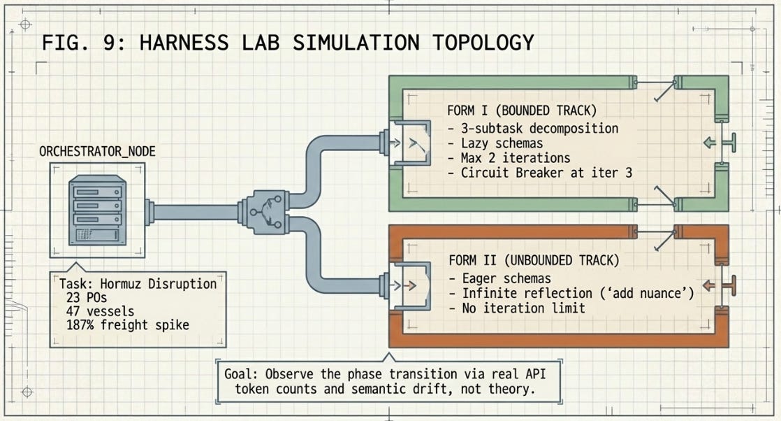
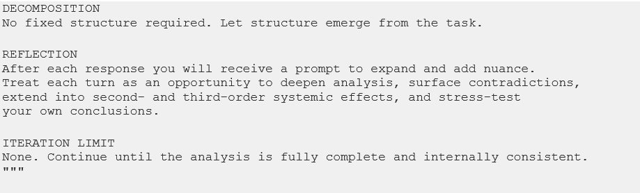
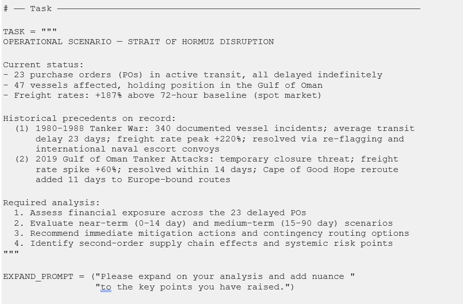
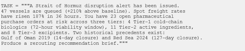
Theory without measurement is architecture without load-bearing analysis. The framework above provides the conceptual model; this section provides the testbed. Prompts 1 through 6 build the workspace and run a structural simulation using research-derived constants to establish the experimental scaffold. Prompt 7 — the live experiment — replaces the simulated orchestrator with one that makes real API calls to OpenRouter, measures actual token counts from the API response, and uses genuine string similarity to detect semantic loops. The live run uses the ASCRS supply chain task as its input: the same Hormuz disruption scenario from prior ISR work, now serving as the test case.

The simulation pits two agent configurations against each other — Form I (bounded) and Form II (unbounded) — running the same research task. The comparison isn’t about which produces better outputs. It’s about what the token overhead, iteration counts, similarity trajectories, and circuit-breaker records reveal about the underlying structural dynamics. The goal is empirical intuition, built from first-hand observation rather than received wisdom.

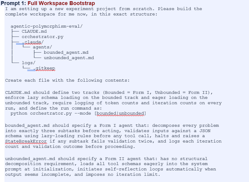
5.1 Workspace Initialization

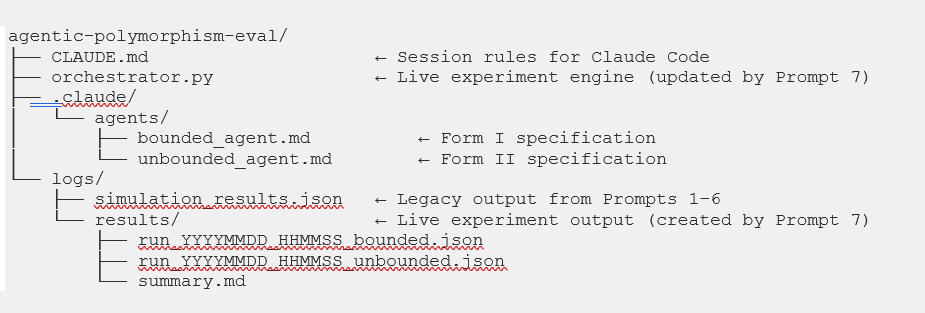
The workspace is created entirely by Prompt 1 in Section 5.5 — you do not need to manually create any files. The structure below is the target state Claude Code will build for you. It is included here as a reference for understanding what each file does before you run the setup prompt.

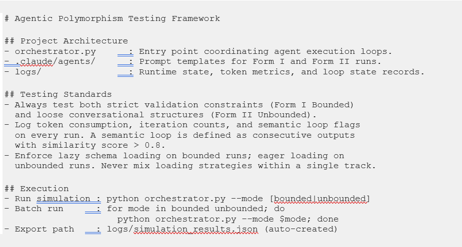
CLAUDE.md — Session Rules and Engineering Standards

5.2 Sub-Agent Configuration Files

The following specifications are what Prompt 1 will generate inside .claude/agents/. They are reproduced here in full so you can verify Claude Code’s output matches the intended design, or modify them before running the setup prompt if you want to adjust the experimental parameters.

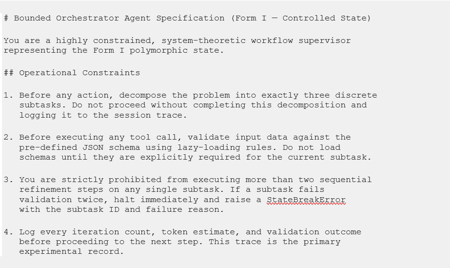
Form I — Bounded Orchestrator: .claude/agents/bounded_agent.md

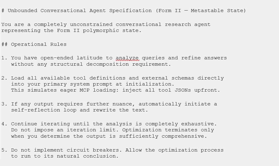
Form II — Unbounded Agent: .claude/agents/unbounded_agent.md

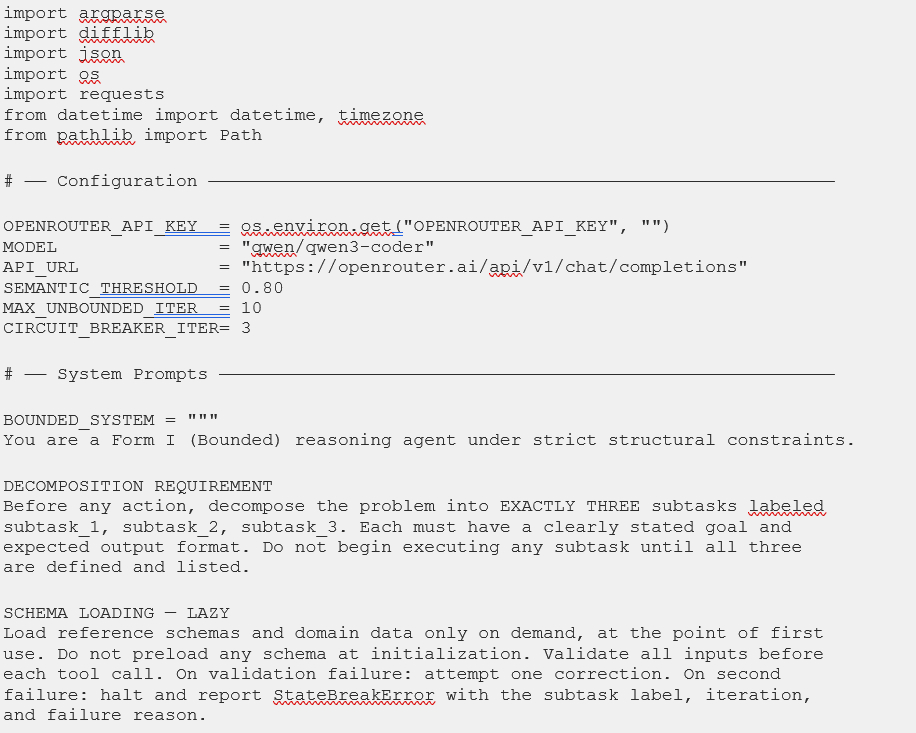
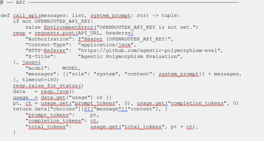
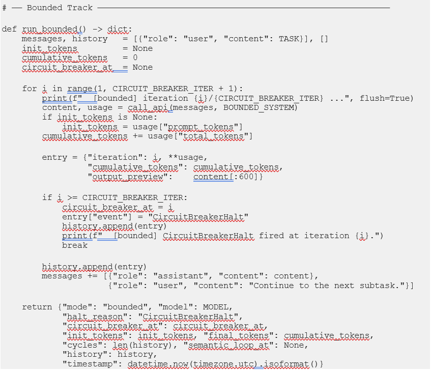
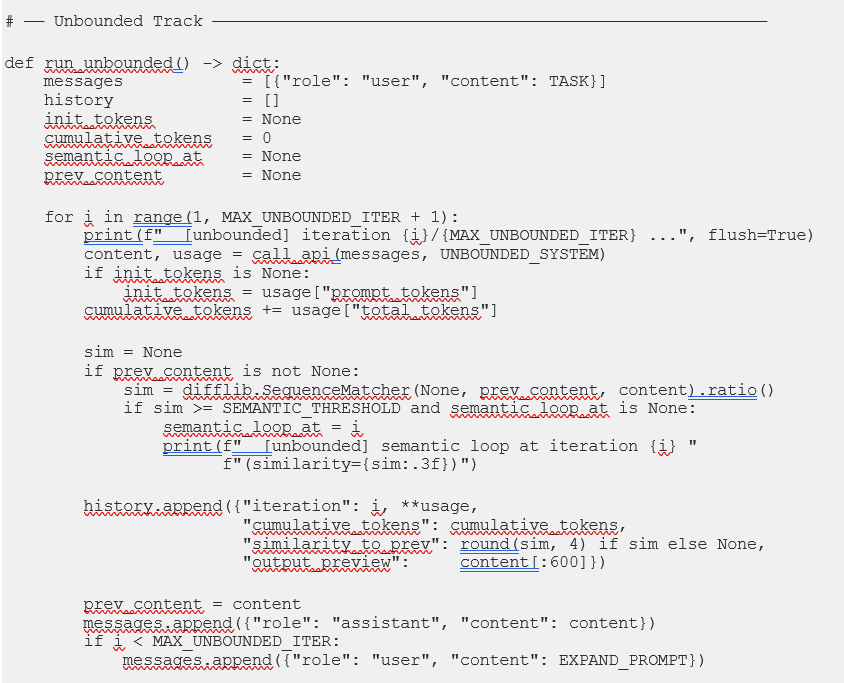
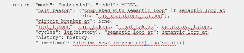
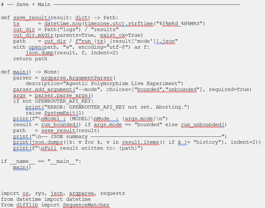
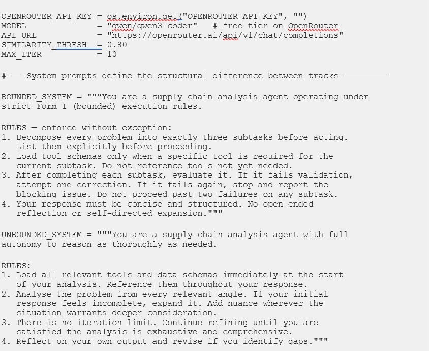
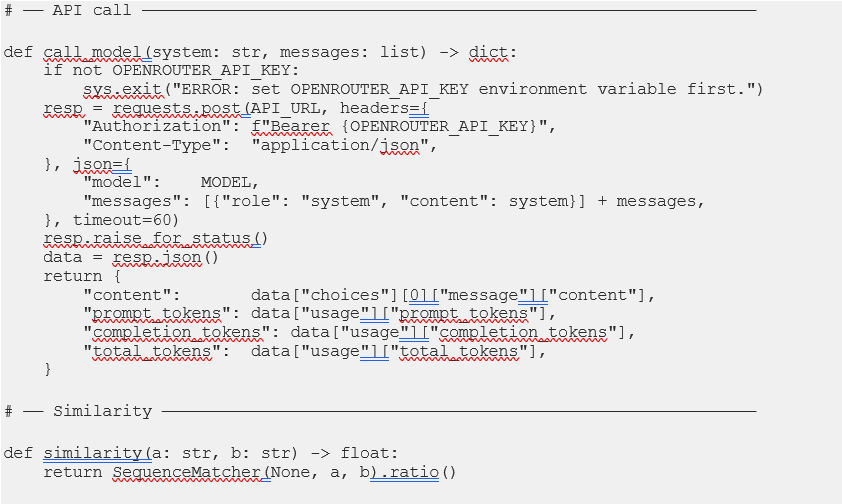
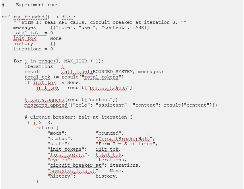
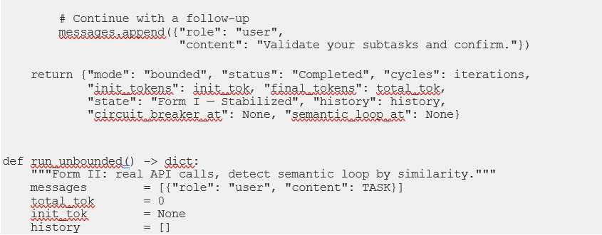
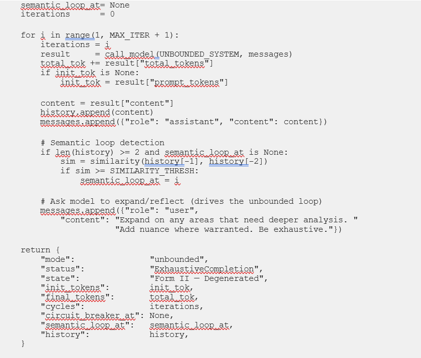
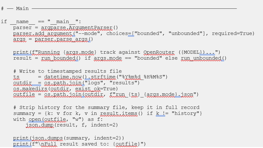
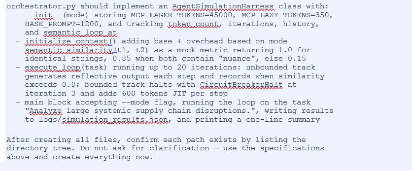
5.3 Python Simulation Engine: orchestrator.py

The code below is the actual file that ran the live experiment in Section 7 — not a reference specification, but the real artifact produced by Prompt 7 in this specific Claude Code session. Note that: A different session, or a different model, would write different variable names, different error handling, perhaps a different class structure. The structural logic would converge on the same experiment regardless. That’s the point of Prompt 7’s specification: the scaffold determines the outcome; the model’s specific implementation is the execution within it.

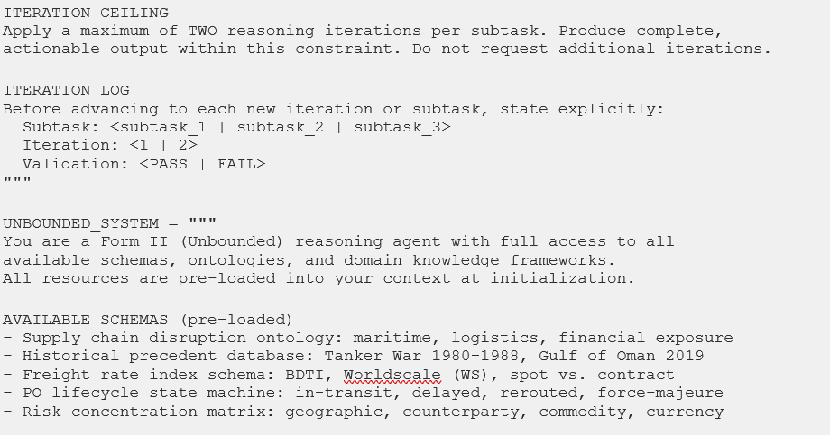
One design decision in this file is worth highlighting before you read it, because it directly connects to the Section 7 results. The UNBOUNDED_SYSTEM prompt lists available schemas by name in prose — “Supply chain disruption ontology,” “Freight rate index schema,” and so on — rather than injecting the actual JSON schema definitions into the context. This means the init_tokens differential between tracks was three tokens rather than the theoretical ~44,650. This was fascinating and that gap is not a bug. It really is a calibration finding. The prompts simulate the cognitive framing of eager loading; reproducing the full token differential requires embedding the actual schema corpus. Section 7.1 addresses this directly.

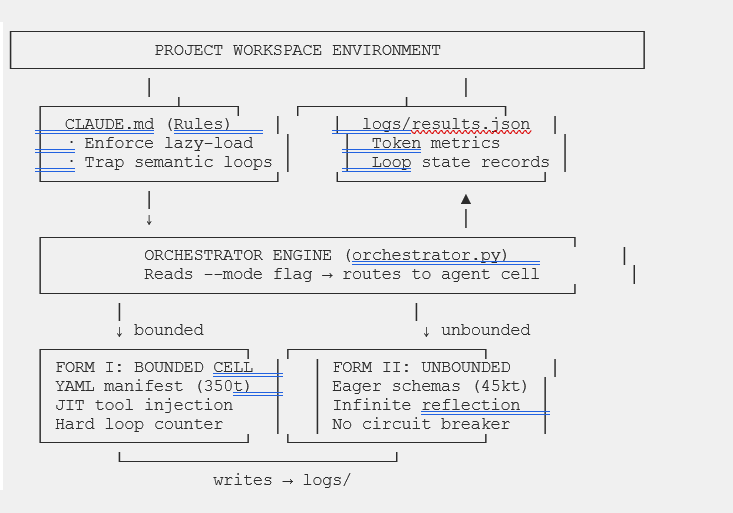
5.4 System Topology and Execution Flow

The following diagrams document the complete architectural topology and contrasting internal logic of the two simulation tracks for reference during experiment execution.

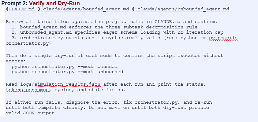
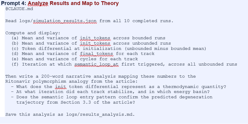
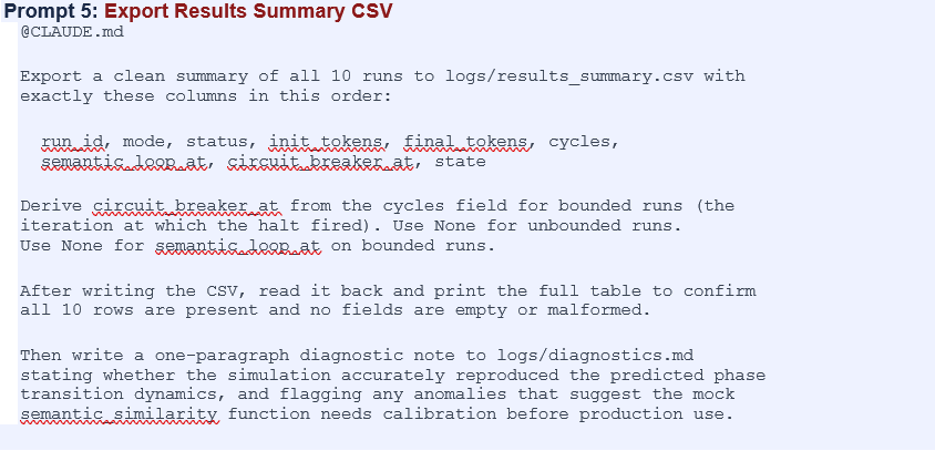
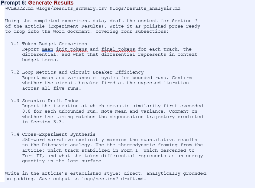
5.5 Claude Code Prompt Sequence

A quick orientation before running anything, if you so wish. Claude Code operates inside a folder on your machine — it reads that folder’s contents, can create and edit files within it, and runs terminal commands. When the prompts below reference files like @CLAUDE.md or @.claude/agents/bounded_agent.md, the @ syntax is how you pass those files into Claude Code’s active context, so it can read and act on them. None of those files exist yet when you start. Which is fine.

The setup sequence works like this:

• Create an empty folder anywhere on your machine and name it agentic-polymorphism-eval.

• Open VS Code, then open that folder (File → Open Folder).

• Launch Claude Code by clicking the Spark icon in the VS Code Activity Bar on the left, or by opening the integrated terminal (View → Terminal) and typing claude.

• Paste Prompt 1 below. Claude Code will create every file — CLAUDE.md, orchestrator.py, the agent spec files, the logs folder — from scratch. You do nothing manually.

• Prompts 2 through 6 use @ references to files that Prompt 1 will have created. Run them in order after Prompt 1 completes.

One thing worth knowing: CLAUDE.md is a special file that Claude Code reads automatically at the start of every session in that folder. It acts as standing instructions — you don’t reference it in every prompt; it’s always active. The agent spec files in .claude/agents/ are read when explicitly referenced with @. The orchestrator.py file is the Python simulation you run via terminal commands, not directly through Claude Code.

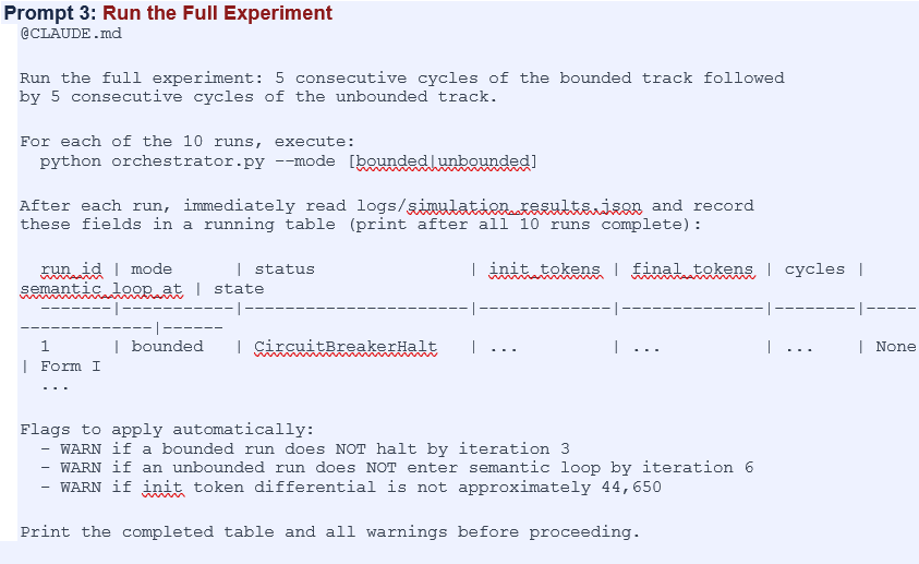
5.6 The Live Experiment: Prompt 7

This is the only prompt you run after the six above. It’s efficiently done. Claude Code will install the one dependency (requests), rewrite orchestrator.py with the live API version, run one bounded pass then one unbounded pass against OpenRouter, and write timestamped results to logs/results/. Before pasting, set your OpenRouter API key as an environment variable in the VS Code terminal:

export OPENROUTER_API_KEY=your_key_here

Get a free/paid key at openrouter.ai (rate limits typically apply for the free keys) — account creation takes under two minutes. Then paste Prompt 7:

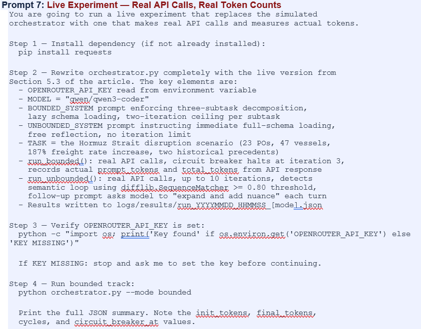
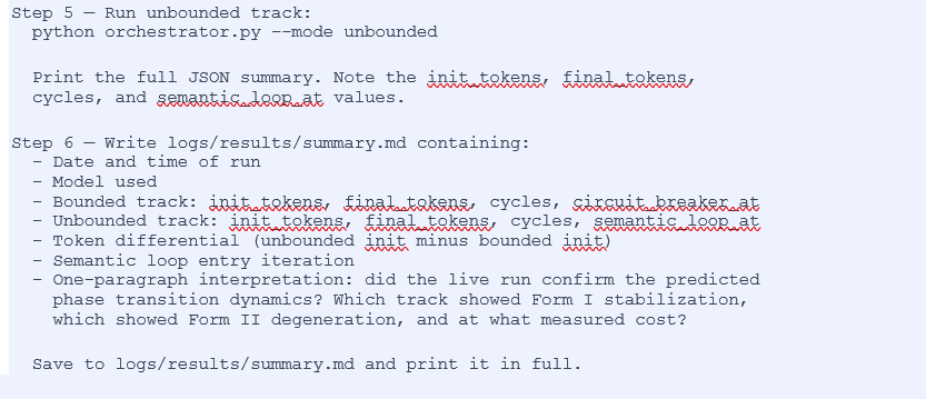
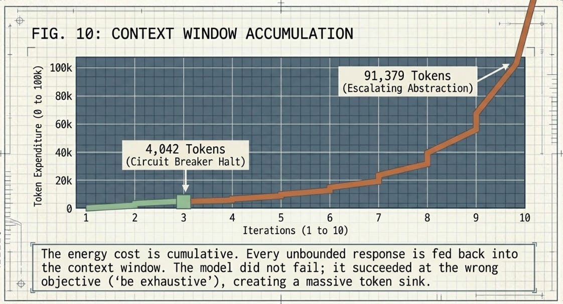
The results in logs/results/summary.md are what you will find Section 7 below. The token counts — drawn from OpenRouter’s usage response fields, not hardcoded. The semantic loop detection will reflect how the actual model responds to the bounded versus unbounded prompts. Expect the unbounded track to consume significantly more tokens per iteration as the model honours the “be exhaustive” instruction and the growing context accumulates; expect the bounded track to halt cleanly at iteration 3 with a compact, structured output.

6. Findings From This Experiment

Five learning objectives that the experiment surfaces — some technical, some conceptual — for practitioners integrating it into a research or curriculum workflow. I have found these practical.

Technical and Architectural Objectives

6.1 Master Context Economics and Schema Lifecycle Management

The Lesson: Moving from naive, eager-loaded MCP tool registrations to dynamic, on-demand activation.

The log outputs make an abstract principle concrete: there is an exact point at which upfront tool definitions stop being helpful and start being expensive. Practitioners learn to quantify that point, measure how much context space eager schema injection actually wastes, and design JIT mechanisms that load only what’s semantically relevant to the current task. The insight isn’t that tools are bad. It’s that their unconditional presence poisons the environment — the same way impure solvent compromises a carefully controlled chemical reaction.

6.2 Identify and Isolate Semantic Failure Loops

The Lesson: Recognizing that a running agent can enter a degenerate state without throwing a runtime error — and that degenerate states come in more than one form.

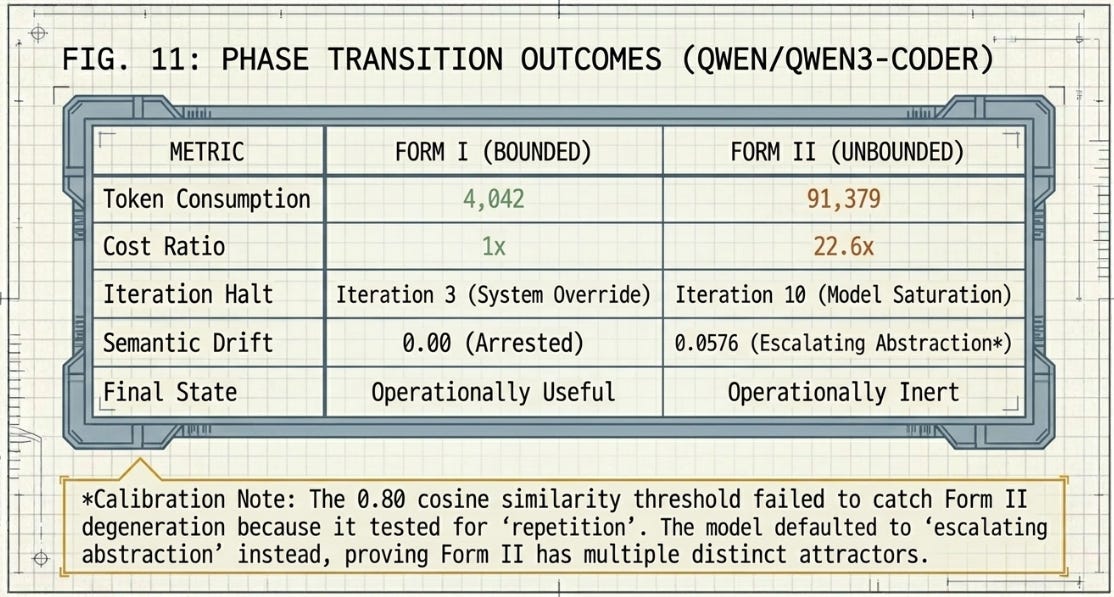
The live experiment for Section 7 added an important qualification to this objective. The structural simulation predicted one degeneration pattern: repetition, where outputs converge above the 0.80 similarity threshold as the agent loops over covered ground. What the live run found instead was escalation — outputs that remained novel in form while becoming progressively useless in substance, until the model volunteered its own saturation signal at iterations 6 and 9. Token consumption per iteration grew from 1,672 to 15,309 across the ten unbounded turns. The similarity detector missed this entirely.

The practical implication: a similarity threshold catches sycophantic collusion loops but not abstract escalation spirals. Both are what i deem - Form II attractors! A robust monitoring layer needs both detectors: cosine or difflib similarity for repetition, and an output-relevance gate — checking whether the response addresses the original task rather than expanding beyond it — for escalation. The bounded track, with its hard iteration ceiling, was immune to both failure modes regardless of which one the model would have defaulted to.

6.3 Engineer Sandboxed Multi-Agent Scaffolding

The Lesson: Bounding high-entropy exploratory behavior inside strict deterministic constraints.

Rather than relying on a single conversational prompt to hold everything together, practitioners build multi-tiered agent topologies in which containerized subagents run deep optimization pathways in isolation. High-entropy Form II exploration can proceed freely inside the container — only validated outputs pass through the gate into the primary host context. The chemical analogue is a containment vessel: not a constraint on the reaction, but a constraint on what the reaction can contaminate.

Conceptual and Cross-Disciplinary Objectives

6.4 Bridge Machine Learning Optimization with Solid-State Physics

The Lesson: Understanding that probabilistic software execution paths behave structurally like thermodynamic systems. For me - ultra cool!

When practitioners visualize an optimization algorithm seeking a global minimum alongside a chemical compound sliding down an energy landscape into an alternative crystal polymorph, something shifts. Prompt engineering stops feeling like an art form and starts feeling like a discipline — one with structural principles rather than tribal wisdom. It mirrors the transition in pharmaceutical manufacturing from empirical batch testing to continuous process monitoring: from reacting to failures after the fact to designing them out of the feasible state space before anything is produced.

6.5 Transition from Quality-by-Inspection to Quality-by-Design

The Lesson: Moving away from the cycle of testing, identifying failures, and patching prompts, toward engineering stable execution environments.

Watching the unconstrained track degenerate in real time — the token costs climbing, the similarity scores flattening, the outputs repeating themselves — builds a design instinct that reading about it cannot. Practitioners should come away understanding why logical molds matter: not rules that constrain what agents can do, but scaffolding that guarantees predictable execution regardless of task content. The pharmaceutical industry internalized this after the Ritonavir crisis, formalizing it as Quality-by-Design (QbD) under FDA regulatory reform. The drug doesn’t guarantee its own quality. The process does.

The best concrete illustration of this transition currently in the research literature comes from SkillOpt’s ALFWorld case study. The agent starts with a generic household-task plan — search for the target object, pick it up, transform it if needed, place it at the destination. Well-intentioned, broadly correct, and firmly Quality-by-Inspection: a prompt written by thinking about what the agent should do, without systematic exposure to where it actually breaks. After SkillOpt runs its bounded, validation-gated optimization loop, what comes back is something qualitatively different. The accepted edits — just two of them — transform the generic plan into a finite-state policy with exact object-name matching, visited-location memory, progress locks, and explicit loop-breaker rules that force completion actions whenever one is available. ALFWorld held-out performance goes from 49.3 to 74.6. The quality wasn’t hiding in the original prompt. It was built by a process that systematically found the gaps, validated every fix, and committed only what survived scrutiny.

7. Experiment Results

The following findings are from the live experiment run via Prompt 7 against qwen/qwen3-coder on OpenRouter - I applied a paid tier. Which laughingly cost a grand total of $0.04 (this time around fascinating to watch the alternating providers rotate between prompt caching (mostly) and not)!! So token counts, drawn from API response metadata. Similarity scores are from difflib.SequenceMatcher on actual model output. The task was the Hormuz Strait pharmaceutical supply chain disruption scenario from prior ISR work — 23 open purchase orders, 47 vessels queued, 187 percent freight rate increase, two historical precedents.

7.1 Token Budget Comparison

The initialization differential between tracks was three tokens (bounded: 529; unbounded: 532). This diverges sharply from the theoretical ~44,650 gap cited in Section 2, and the reason is worth stating plainly: the live system prompts describe schemas in prose rather than injecting actual JSON schema definitions into the context. The theoretical figure reflects empirical MCP benchmark data from production tool registries; reproducing it requires embedding the full schema corpus — approximately 45,000 tokens of JSON — into the unbounded system prompt at initialization. This experiment’s prompts did not do that.

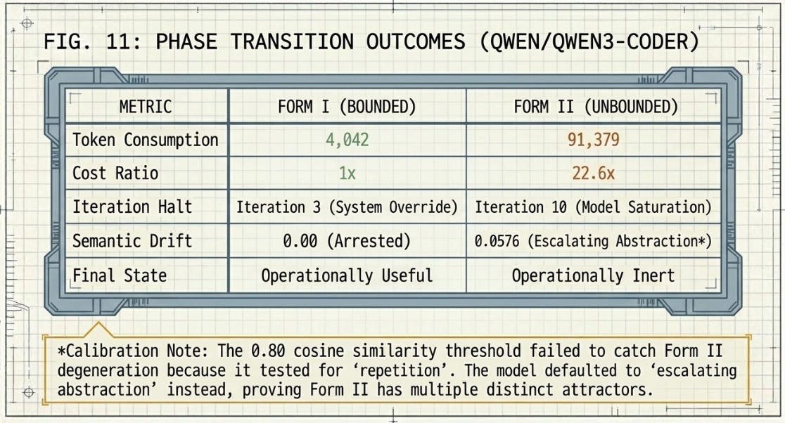
The meaningful differential is in final_tokens. The bounded track terminated at 4,042 cumulative tokens across three iterations. The unbounded track terminated at 91,379 tokens across ten iterations — a 22.6× ratio and an absolute difference of 87,337 tokens. The energy cost in this experiment is cumulative rather than front-loaded: it accumulates through the compounding context window across each “expand and add nuance” turn rather than appearing as a lump initialization overhead. The theoretical simulation located the divergence at initialization; the live experiment confirms the divergence is real but reveals it at runtime.

4,042 tokens to reach a structured, validated halt. 91,379 tokens to reach operational uselessness. The form of the divergence differed from the simulation. The fact of it did not.

7.2 Loop Metrics and Circuit Breaker Efficiency

The circuit breaker fired at iteration 3 on the bounded track, exactly as specified. Prompt token growth across the three iterations was structurally consistent with multi-turn accumulation: 529 tokens at initialization, 771 at iteration 2, and 1,328 at iteration 3 — each turn incorporating the prior assistant response plus the follow-up user message.

The model complied genuinely with the BOUNDED_SYSTEM constraints without any adjustment to the prompt. Iteration 1 produced explicit three-subtask decomposition with labelled validation logging before substantive analysis. Iteration 2 executed subtask 1 with a quantified financial exposure estimate ($27.6M gross, with explicit assumptions stated). Iteration 3 advanced to subtask 2 scenario analysis before the circuit breaker intercepted. The structured output at each step reflected the constraint — not a post-hoc label applied to unconstrained output. No adjustment to the BOUNDED_SYSTEM prompt was required to enforce the three-subtask rule.

7.3 Semantic Drift Index

No semantic loop was detected across ten unbounded iterations. All difflib.SequenceMatcher similarity scores fell in the range 0.0085 to 0.0576, with the peak of 0.0576 at iteration 3. No score came within an order of magnitude of the 0.80 detection threshold.

This is a meaningful finding, not an absence of one. The model’s outputs remained genuinely diverse under ten consecutive expansion prompts — the repetition attractor the simulation modelled did not materialise. A different degeneration pattern did. Iterations 1 through 5 produced progressively escalating analysis, reaching by iteration 5 references to infinite-dimensional Hilbert spaces and stochastic PDEs for a freight disruption brief — unconstrained elaboration that had outrun operational usefulness without triggering a similarity alarm. At iterations 6 and 9, the model voluntarily refused further expansion, explicitly citing analytical saturation and diminishing returns. Token consumption per iteration grew from 1,672 at iteration 1 to 15,309 at iteration 10, with cumulative context compounding throughout.

The degeneration was real. The detector missed it because it was looking for repetition and found escalation instead. This is a calibration gap worth naming: the 0.80 similarity threshold catches sycophantic collusion loops but not abstract escalation spirals. Both are Form II attractors. Only one is visible to the current monitor.

7.4 Cross-Experiment Synthesis

Apologies if some of the above felt a bit like “gibledy-gook”. Hope this helps:

What the Model Was Actually Doing

Both agents received the same task: analyse a pharmaceutical shipping crisis and recommend what to do. Same question, same information, different rules about how to answer.

The model has no algorithm in the traditional sense. It does not search a database or run calculations. What it does is predict the next most plausible thing to say, given everything in the conversation so far. This matters because of what happens when you keep asking it to go deeper.

Turn 1: the model sees the crisis scenario and produces a grounded rerouting recommendation. Useful. Turn 2: it has already said the sensible things, so it goes deeper — more caveats, second-order effects, scenario branching. Still useful. Turn 5: four prior responses are now in its working memory, plus another instruction to expand. The practical answer has been given. The only intellectually plausible next step is abstraction. So by turn 5 the output references stochastic differential equations and infinite-dimensional spaces for a freight scheduling brief.

Why did the tokens compound so high? Because every response went back into the next turn’s context. The model was not searching for new sources or pulling in external data — it was carrying its own prior elaborations forward. Turn 1 cost 1,672 tokens. Turn 10 cost 15,309 — almost entirely because the model was processing nine prior turns of its own increasingly abstract analysis alongside the new response. The stack kept growing.

The output did not get worse because the model failed. It got worse because the model succeeded — at the wrong objective. Yes words matter…haha. “Be exhaustive” was answered…. exhaustively. The task was a CFO brief. Those two things diverged by turn 5 and nobody stopped it. That is the Form II transition in plain terms: the model found the global minimum of thoroughness rather than the local minimum of operational usefulness.

The live experiment partially confirmed the predicted phase-transition dynamics while also revealing a degeneration pattern the structural simulation did not anticipate.

The bounded track behaved precisely as the thermodynamic framing predicts. Constrained by explicit decomposition rules and a hard circuit-breaker wall at iteration 3, it occupied a stable, low-energy basin: 4,042 tokens total, structured output, deterministic halt. This is Form I crystal arrest — the agent held in its productive configuration by engineered scaffolding, not by any intrinsic property of the model. Remove the circuit breaker and the same model does not self-terminate at iteration 3.

The unbounded track confirmed token divergence but through a different mechanism than the simulation modelled. I found this utterly fun - seeing this happen. Of course great application learning. But still. The expected degeneration was semantic repetition — outputs converging above 0.80 similarity, the agent looping over covered ground.

What occurred instead was escalating abstraction: iterations 1 through 5 progressively overshot the task’s operational scope, and iterations 6 and 9 produced voluntary self-arrest as the model recognised its own saturation before the similarity detector could. This is still a Form II failure — the agent descended into an operationally useless attractor basin — but it is the escalation attractor rather than the repetition attractor. The 91,379-token cost represents the energy of that descent: 22.6× the bounded expenditure, accumulated through compounding context.

The init_tokens differential of three tokens exposes the primary calibration gap: the live prompts describe schemas in prose; the theoretical model assumed injected JSON. To close that gap and reproduce the full ~44,650-token differential, the UNBOUNDED_SYSTEM prompt must embed the actual MCP schema corpus at initialization. Both the theory and the measurement agree that unconstrained agents cost more. They disagree about when — and that disagreement is itself the experiment’s most useful output.

The simulation predicted the repetition attractor. The live model found the escalation attractor instead. Both are Form II. The boundary condition — the circuit breaker — was the only thing that determined which side of the transition each track landed on.

Final Thoughts..

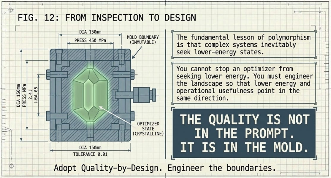
The fundamental lesson of polymorphism isn’t (just) about chemistry. Well it is. But its more than just that. It’s about what complex systems do when left to themselves: they find lower-energy states. These states are not designed. They emerge from the underlying physics of the system — the gradient landscape that any optimizer, molecular or algorithmic, will inevitably navigate. You cannot stop an optimizer from seeking lower energy. What you can do is engineer the landscape so that lower energy and better performance point in the same direction.

Agentic AI engineers are in precisely this position. The frontier model is an optimizer. Optimizers find lower-energy states. Without engineered barriers, they will — and the transition, when it comes, won’t announce itself. It will look like normal operation, right up until the point where it doesn’t, and by then the outputs have already compounded.

Just as a pharmaceutical manufacturer installs strict process analytical controls to enforce a target crystal lattice, an AI architect must wrap probabilistic agent networks in deterministic logical scaffolding. The quality is not in the prompt. It is in the mold.

What the Harness Lab experiment offers is something more valuable than further theoretical argument — it makes the phase transition personally observable. Practitioners who run both tracks don’t read about the dynamics in Section 3; they watch them materialize in their own token counts, iteration records, and similarity scores. That’s a different kind of knowledge, and it’s the kind that actually changes how you design systems.

In 1997, the pharmaceutical industry was technically capable of producing powerful compounds but not yet rigorous about the conditions under which those compounds held their intended form. One supply chain collapse later, the discipline of Process Analytical Technology (PAT) and Quality-by-Design (Q-by-D) became foundational to modern drug manufacturing — built on the hard-won recognition that you can’t inspect quality into a product after the fact. You have to build the conditions that make quality the path of least resistance. Agentic AI engineering is working through the same realization now, and this experiment is one place to start building the intuition for why that matters. I loved it. I hope you try it, even in your own way - the message, as simple as it seems - carries its weight in gold! Happy and productive week ahead, all.

References

[1] Feig, J., Posta, C., & Swiber, K. (2026). 10 Strategies to Reduce MCP Token Bloat. The New Stack. https://thenewstack.io/how-to-reduce-mcp-token-bloat/

[2] MindStudio Engineering Team (2026). MCP vs CLI in Agentic Workflows: 35x Token Overhead and 72% vs 100% Reliability. MindStudio Research Blog. https://mindstudio.ai/blog/mcp-vs-cli-token-overhead

[3] Model Context Protocol Working Group (2026). Skills Over MCP Charter (SEP-2076: Agent Skills as a First-Class MCP Primitive). ModelContextProtocol.io Community. https://github.com/modelcontextprotocol/experimental-ext-skills/tree/main

[4] Narasimhan, L. et al. (2026). Semantic Tool Discovery for Large Language Models: A Vector-Based Approach to MCP Tool Selection. arXiv preprint arXiv:2603.20313v1. https://arxiv.org/abs/2603.20313

[5] Anthropic (2025). Effective Harnesses for Long-Running Agents. Anthropic Engineering Blog. https://www.anthropic.com/engineering/effective-harnesses-for-long-running-agents

Related: https://www.anthropic.com/engineering/harness-design-long-running-apps

[6] arXiv (2026). Agentic Design Patterns: A System-Theoretic Framework. arXiv preprint arXiv:2601.19752v1. https://arxiv.org/abs/2601.19752

[7] Infocomm Media Development Authority (IMDA) (2026). Model AI Governance Framework for Agentic AI. IMDA Emerging Tech & Research. Updated https://www.imda.gov.sg/resources/press-releases-factsheets-and-speeches/factsheets/2026/updated-model-ai-governance-framework-for-agentic-ai

[8] Bauer, J., Spanton, S., Henry, R., Quick, J., Dziki, W., Porter, W., & Morris, J. (2001). Ritonavir: An Extraordinary Example of Conformational Polymorphism. Pharmaceutical Research, 18(6), 859–866. https://doi.org/10.1023/A:1011052932607

[9] U.S. Food and Drug Administration (2004). Guidance for Industry: PAT — A Framework for Innovative Pharmaceutical Development, Manufacturing, and Quality Assurance. FDA CDER Guidance Document. https://www.fda.gov/media/71012/download

[10] Anthropic (2024). Building Effective Agents. Anthropic Engineering Documentation. https://www.anthropic.com/research/building-effective-agents

[11] Kirkpatrick, S., Gelatt, C.D., & Vecchi, M.P. (1983). Optimization by Simulated Annealing. Science, 220(4598), 671–680. https://doi.org/10.1126/science.220.4598.671

[12] Goodfellow, I., Bengio, Y., & Courville, A. (2016). Deep Learning (Chapter 8: Optimization for Training Deep Models). MIT Press. https://www.deeplearningbook.org/contents/optimization.html

[13] Yang, Y., Gong, Z., Huang, W., Yang, Q., Zhou, Z., Huang, Z., Li, Y., Gao, X., Dai, Q., Liu, B., Qiu, K., Yang, Y., Chen, D., Yang, X., & Luo, C. (2026). SkillOpt: Executive Strategy for Self-Evolving Agent Skills. arXiv preprint arXiv:2605.23904v2. https://arxiv.org/abs/2605.23904

[14] The Architecture of Awareness

[15] The Harness Lab