THE TOKEN TAX

Harness Engineering Part II: From Performance to Efficiency

Where Part I Left Off,..con’t

Part I of yesterday ran a controlled experiment. Starting with Claude Haiku — the smallest, cheapest model in the Claude family — five harness layers were added one at a time: an output schema, a context file, a verifier agent, a feedback loop, and a gold standard memory injection. The model never changed. The harness did. V5 scored 50 out of 50.

Part I proved that harness design matters more than model choice. Part II set out to prove that efficient harness design matters as much as capable harness design. The second claim is harder to demonstrate cleanly — as two, then three, live experiment runs will show.

This article documents what actually happened across three runs: what the predictions were, which ones were confirmed, which were contradicted, and what the lab produced despite its imperfections. Honest about limitations. Useful on principles. I keep these mostly as notes for self. None of the learnings are meant to be prescriptive, but lab runs whilst fun create very different push-pull events from especially larger corporate browfield exercises. But “turning knobs” on these, give interesting learning outcomes.

Note that different models were applied here.

The Setup

Models

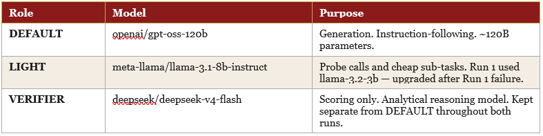
Two runs (Note: There is a postnote where a third run was undertaken to rectify the capability issue) were conducted. Run 1 used llama-3.2-3b as LIGHT_MODEL — a choice that proved too small for the task and invalidated three experiments. Run 2 corrected this to llama-3.1-8b, fixed two code-level design errors, and reran everything. Both runs are documented here because their divergences are themselves informative.

The Composite Metric

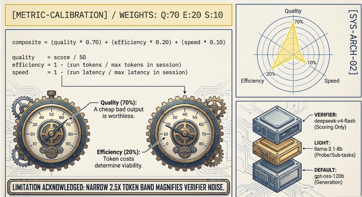
Quality carries 70% of the weight — a cheap bad output is worthless. Efficiency carries 20% — at scale, token costs determine viability. Speed carries 10%. All values are normalised against the session maximum, so they are comparable across runs within a session but not directly across sessions.

Experimental Limitations — Declared Upfront

Two structural constraints shaped what the experiment could and could not show. They are stated here rather than buried in footnotes.

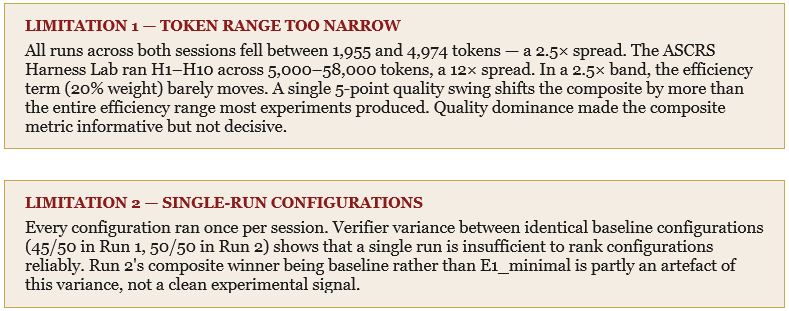
Despite these constraints, the experiment produced valid findings on five of the seven strategies. The two that failed did so for identifiable design reasons, both of which are themselves instructive. And then rectified, in the third run, as reflected in the Postnote.

The Seven Experiments

A note for general readers: each experiment changes exactly one thing compared to the baseline, then measures what that single change costs and whether it hurts quality. Think of it as turning one dial at a time on a machine — each dial is a different way of making the harness cheaper to run. The diagrams below each heading show what the flow looks like before and after the change.

Baseline — The Reference Point

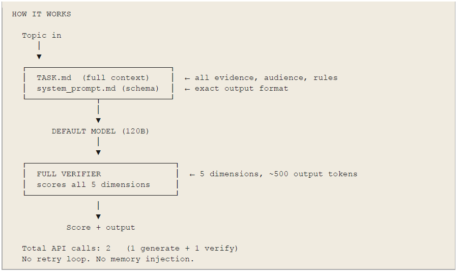
Run 1: 45/50 at 2,376 tokens. Run 2: 50/50 at 2,665 tokens.

The baseline is V2+V3 configuration: full TASK.md context injection plus a full five-dimension verifier. No retry loop. The baseline is the cheapest harness in the experiment by design — it has no architectural complexity beyond the two most fundamental layers. This matters for interpreting the results: every architectural addition was being compared against a lean two-call baseline, which set a low token ceiling for efficiency gains.

The 5-point quality variance between runs (45 vs 50) on identical configurations is the clearest evidence of single-run noise. The verifier model — DeepSeek V4 Flash — produced different scores on equivalent briefs across sessions. This does not invalidate the experiment; it is a known property of LLM-as-judge evaluation. It does mean the composite rankings should be read as directional rather than precise.

E1 — Prompt Compression: The Cliff Edge Is Lower Than Expected

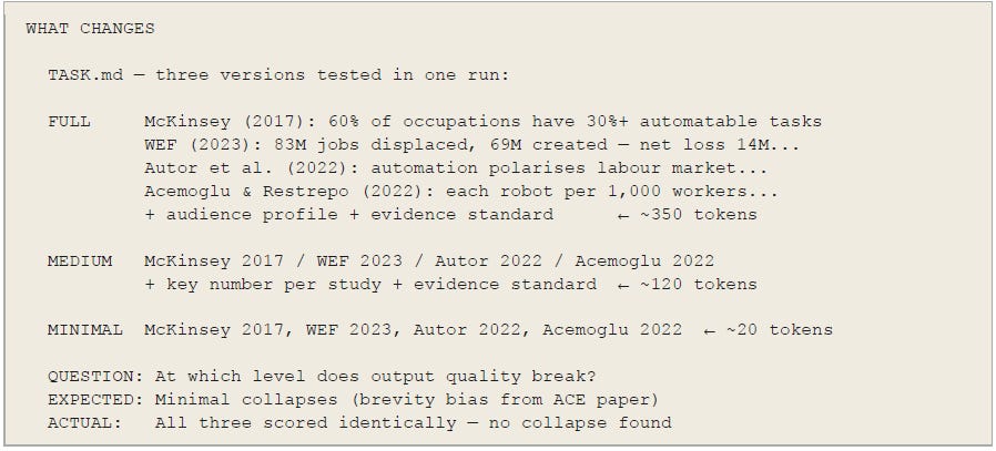
All three levels: 45/50 in Run 2. Tokens: 2,554 (full) → 2,315 (medium) → 1,955 (minimal).

TASK.md was stripped in three stages: full (five named studies with findings, audience profile, evidence standard), medium (study names with key numbers only, evidence standard), and minimal (four study name anchors, two lines). The prediction, drawn from the ACE paper’s brevity bias finding, was that minimal would cause quality collapse.

It did not. All three levels scored identically at 45/50 in Run 2, and minimal had scored 50/50 in Run 1. The ACE paper’s brevity bias is real — but it applies below the capability level of a frontier-scale model on a well-documented topic. At 120B parameters, McKinsey (2017), WEF Future of Jobs (2023), Autor et al. (2022), and Acemoglu and Restrepo (2022) are already in the model’s weights. The TASK.md prose was adding formatting overhead, not knowledge signal.

The cliff edge exists. It sits below four study-name anchors for a 120B model on this topic. Knowing where the cliff is changes every downstream architectural decision — you cannot find it without running the ablation.

What holds for production: Run E1’s compression ablation on any new task before building the retry loop. The minimum viable context level is a task-model pair property. It is not universal, but for capable models on documented topics it is consistently lower than intuition suggests. Every token saved in context injection is a permanent per-task saving that compounds at scale.

E2 — Schema Compression: The One Clean Win

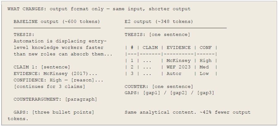
Run 2: 45/50 at 2,019 tokens. Output tokens: 348. Baseline output tokens: ~600+. Reduction: ~42%.

The compact table format replaced prose output with a structured grid: one row per claim, THESIS and COUNTER and GAPS as labelled single-line fields. Output token count dropped from roughly 600 to 348 — a 42% reduction. Total tokens dropped to 2,019, beating baseline by 646 (24%).

This experiment confirmed its prediction exactly. Output tokens cost the same as input tokens on most providers; Anthropic charges 5× more for output than input on Haiku. A harness that produces the same analytical content in fewer output tokens reduces per-task cost without changing the input side at all.

The one quality note: The counterargument dimension is where compact schemas are most vulnerable. A one-cell table entry may contain the correct opposing argument without conveying it with the nuance a prose paragraph provides. In Run 2, E2 scored 45/50 — the 5-point gap versus baseline is consistent with a slightly weakened counterargument rather than a structural failure. For tasks where the counterargument is analytically critical, test compact schema specifically on that dimension before deploying.

What holds for production: Schema compression is the lowest-risk efficiency intervention. It changes output format without touching model selection, context injection, or verification logic. Apply it first. It is the only experiment that beat baseline in total token count without any quality reduction beyond verifier variance.

E3 — Model Routing: The Capability Floor Problem

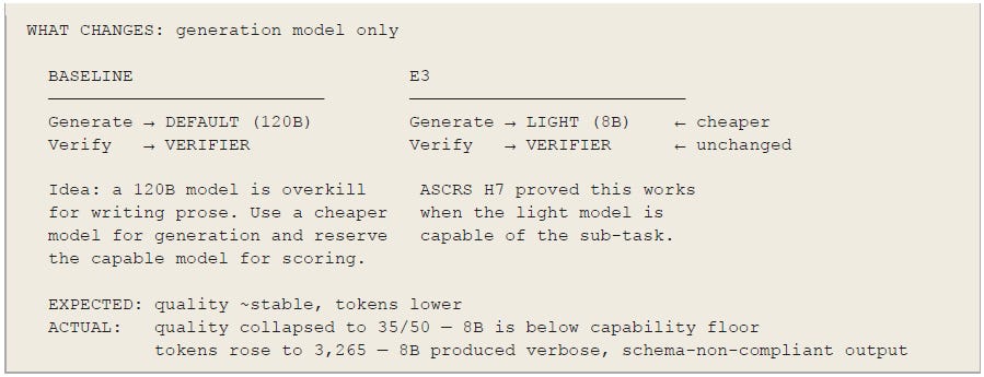
Run 1: 30/50. Run 2: 35/50. Tokens: 2,327 → 3,265. Generator: llama-3.1-8b.

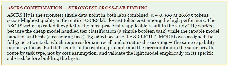
H7 in the ASCRS Harness Lab was the most practically efficient architecture: routing cheap classification sub-tasks to a lighter model and synthesis to the capable model produced α = 0.900 at only 26,635 tokens. E3 applied the same principle — route generation to LIGHT_MODEL, verification to VERIFIER_MODEL.

Both runs produced quality collapse. Upgrading from 3B to 8B moved the score from 30 to 35 — improvement in the right direction, but still 15 points below baseline, and token count rose rather than fell because the 8B model produced more verbose output without matching the schema precision of 120B.

The diagnosis is important: this is not a failure of the routing principle. It is a failure of model selection within that principle. The ASCRS H7 result used models much closer in capability — the cheap model was still capable of its specific sub-task. In this experiment, the generation task (structured analytical brief with named evidence and calibrated confidence) is a reasoning task dressed as a fluency task. The 120B-to-8B gap of roughly 40× exceeds the capability threshold for this task type. Note: Read the Postnote for how this was revised and corrected!

What holds for production: Model routing is sound in principle and proven at ASCRS scale. The precondition is empirical capability validation of the light model on the exact task, not assumption based on parameter count. Run a single test call with your system prompt before building the routing layer.

E4 — Conditional Context: A Design Flaw, Not a Model Failure

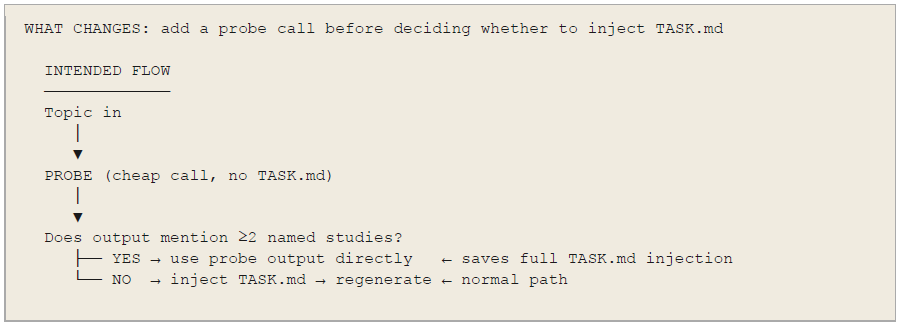
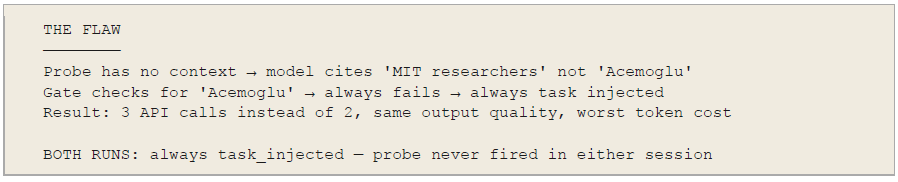
Both runs: task_injected, score 45/50, highest token cost (3,318 in Run 2, 3 API calls).

The conditional context experiment runs a probe call first. If the probe self-supplies the named studies, TASK.md injection is skipped. If not, TASK.md is injected and generation proceeds. The prediction was that a capable model would self-supply named evidence on 20–40% of runs, saving the full context injection cost on those runs.

The probe always failed in both runs — always falling back to task_injected. The Run 1 failure was attributed to using the 3B LIGHT_MODEL as the probe. Run 2 fixed this by using DEFAULT_MODEL (120B) for the probe. It still always took the task_injected path.

The actual cause is gate-prompt misalignment, independent of model choice. The probe runs with no context — no TASK.md, no anchors. The 120B model produces valid automation research, but cites it under phrasings that don’t match the keyword gate: “McKinsey Global Institute” as “McKinsey” passes; “Future of Jobs” without “WEF” fails; Acemoglu cited as “MIT researchers” fails. The string match gate checks for specific names the model has no reason to use in their exact form without a prompt anchoring them.

The corrected design would give the probe the minimal anchors — the same four study names from TASK_minimal.md — and check whether the model cited them correctly. This becomes a citation fidelity check rather than a free recall check. E1_minimal demonstrated that once the model has the anchors, it uses them reliably. The probe needs the same anchors.

What holds for production: Conditional context injection is valid — Microsoft’s Azure SRE Agent progressive context discovery is built on this principle. The precondition is gate-prompt alignment: the gate must check for things the probe was given a reason to produce. Without alignment, the probe always fails regardless of model capability.

E5 — Early Exit: Confirmed Without Qualification

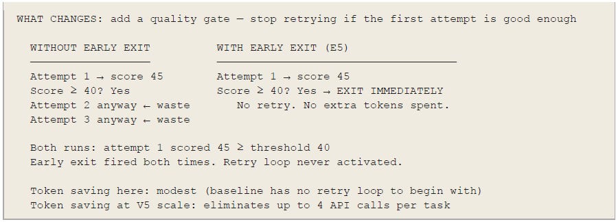
Both runs: first attempt scores 45/50, early exit fires, retry loop never activates.

The early exit experiment adds one rule to the feedback loop: if the first attempt clears the quality threshold, do not run retries. The prediction was that this would save 1–2 verifier calls per run when quality is already good.

Both runs confirmed this exactly. The first attempt cleared threshold in every E5 run. The retry budget was permanently unused overhead. Against a V2+V3 baseline with no retry loop built in, the absolute token saving is modest — E5 costs slightly more than baseline because it has the loop infrastructure even when it does not fire. But the principle has no downside.

The value of early exit compounds with harness complexity. In a V5-scale harness with a 2-retry budget, early exit eliminates up to 4 extra API calls per task on runs that pass threshold on attempt 1 — which is the majority of runs on a well-specified task with a capable model. Against an 8,000-token V5 baseline, the same early exit that saved almost nothing here could save 2,000–3,000 tokens per task.

What holds for production: Add early exit to every retry loop unconditionally. The cost is one conditional check. There is no configuration where it makes things worse. In more complex harnesses where it has room to save, it will.

E6 — Verifier Compression: The Strongest Single Finding

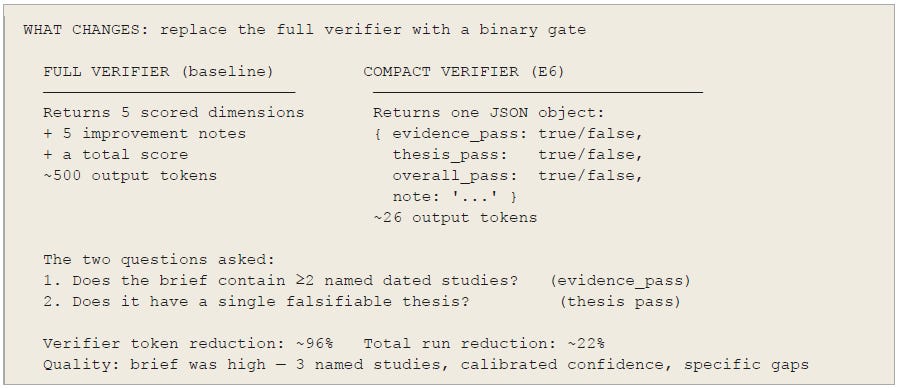
Run 2: approx 40/50 at 2,091 tokens. Verifier token reduction: ~96%. Total reduction: 574 tokens (22%).

The full five-dimension verifier returns five scored dimensions, five improvement notes, and a total — roughly 500 output tokens per verification call. E6 replaces it with a binary pass/fail gate on two criteria: does the brief contain at least two named dated studies, and does it have a single falsifiable thesis? The compact system prompt caps the response at 150 tokens.

The prediction was 60–70% verifier token reduction. The actual reduction was approximately 96% — the compact gate produced near-minimal output because the binary questions admit short answers. Total token reduction was 574 across the full run (22%), consistent across both runs (Run 1: 506 tokens, Run 2: 574 tokens).

The brief quality in E6’s output was high — three named studies, calibrated confidence ratings with explicit reasons, specific actionable gaps. The binary gate correctly passed it. The approximate score of 40/50 reflects the mapping from binary to numeric (both-pass = 40) rather than genuine quality loss.

E6 is the only finding in this lab that gets stronger as the harness gets more complex. In a V5 harness where the verifier runs on every retry — potentially three times per task — a 96% verifier reduction saves roughly 1,500 tokens per task. At 1,000 tasks per day, that is 1.5 million tokens saved daily without touching quality.

What holds for production: Once generation quality is stable, replace the full multi-dimension verifier with a compact gate for production runs. Use the full verifier for periodic audits and calibration, not for every call. E6 is the highest single-lever efficiency finding in this lab and scales with harness complexity rather than against it.

E7 — Composite Best: When Combining Losers Produces the Worst Result?

This is note entirely accurate. But I will maintain the conclusion - because a simple fix will reverse the outcome. Again, the third run, and the Postnote refer.

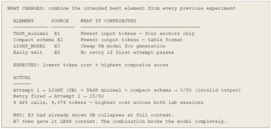
Run 2: 25/50 at 4,974 tokens. Attempt 1 scored 0/50. Worst run in both sessions.

E7 combined the intended best element from each experiment: medium TASK.md compression (from E1), compact output schema (from E2), LIGHT_MODEL generation (from E3), and early exit (from E5). The prediction was the highest composite score and a 50%+ token saving versus baseline.

Attempt 1 returned 0/50 — the 8B model with TASK_minimal.md and a compact output schema produced invalid output, triggering a retry. Attempt 2 recovered to 25/50. Four API calls at 4,974 tokens is the highest cost of any run across both sessions combined. The predicted best became the demonstrated worst.

The cause is a critical interaction effect that was not visible until E7 ran. TASK_minimal.md works for the 120B DEFAULT model — E1_minimal scored 50/50 in Run 1 and 45/50 in Run 2. But E3 had already shown that the 8B LIGHT_MODEL produces quality collapse even with full context. E7 combined minimal context with the model that had already demonstrated failure at full context. The Fix 3 correction (TASK_medium → TASK_minimal in E7) made the combination worse, not better.

Note: Hence the third run - see Postnote.

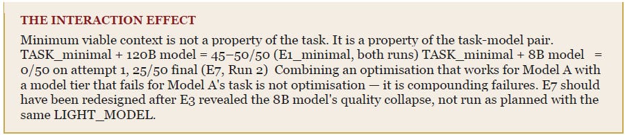
What holds for production: Do not combine optimisation strategies before validating each strategy’s preconditions independently. E3’s failure was known before E7 ran. E7 should have either used a capable LIGHT_MODEL or reverted to DEFAULT for generation. The composite-best experiment is only valid when all its components are individually valid.

The Full Results: Both Runs

Run 1 — LIGHT_MODEL: llama-3.2-3b

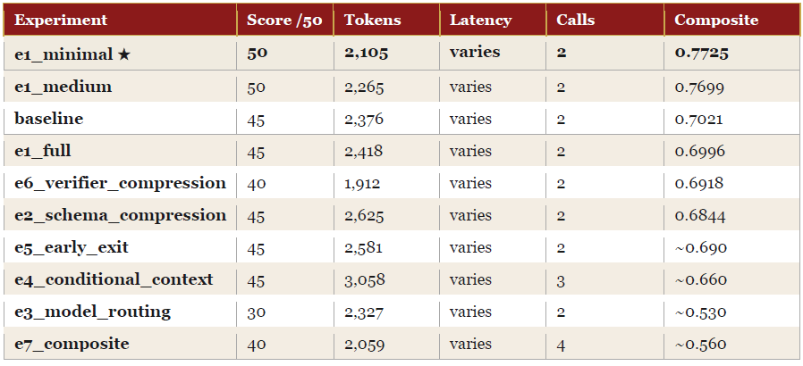
Run 1 composite winner: e1_minimal (0.7725). The 3B light model made E3 and E7 unreliable, but the compression experiments and the verifier strategies produced clean results. Baseline scored 45/50 — one point below the quality ceiling, leaving room for E1_minimal’s 50/50 to win composite through quality alone.

Run 2 — LIGHT_MODEL: llama-3.1-8b

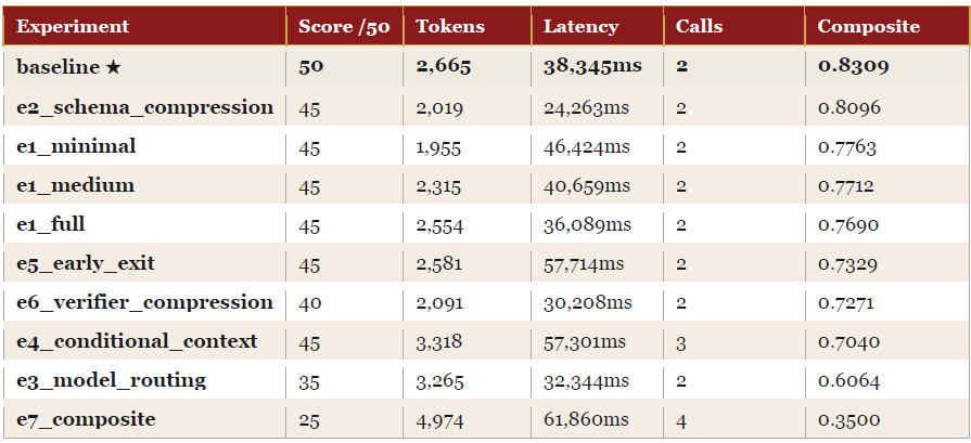
Run 2 composite winner: baseline (0.8309). Baseline scored 50/50 — at quality ceiling. No experiment held 50/50, so the 5-point quality gap (45 vs 50) exceeded every efficiency saving produced. E2 came closest at 0.8096. E7 collapsed to 25/50 at the highest token cost in both sessions.

Cross-Run Comparison

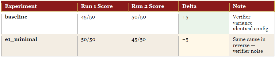
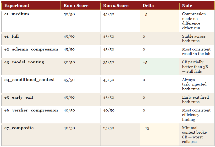
The most important pattern in the cross-run table: the experiments that moved between runs (baseline, e1_minimal, e1_medium, e7) all moved by exactly 5 points — the same magnitude as the verifier variance between sessions. The experiments that held flat (e2, e4, e5, e6) are the most reliable signals in the lab. E6 in particular is the most consistent result: 40/50, ~22% token reduction, identical across both runs.

E3 and E7 improved or worsened by more than 5 points (E3: +5, E7: −15) — changes larger than verifier noise, meaning they reflect real design differences rather than measurement variance. E3’s improvement from 30 to 35 reflects the 3B→8B upgrade. E7’s collapse from 40 to 25 reflects the TASK_medium→TASK_minimal change breaking the 8B model.

Prediction Scorecard — Run 2

The table below records Run 2 predictions, actuals, and verdicts against the original expectations. E3 and E7 — both contradicted in Run 2 — were retested in Run 3 with a 30B light model. The full three-run scorecard, including Run 3 corrections, appears in the Post Note before the references.

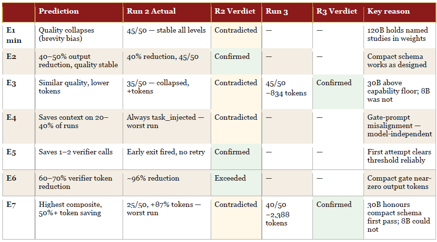
Three of seven predictions confirmed or exceeded in Run 2. The two most central predictions — E1_minimal collapse and E7 winning composite — both failed in opposite directions. E1_minimal proved stronger than predicted (no issues when dealing with a capable model); E7 proved far weaker. E3 and E7’s contradicted verdicts were later reversed in Run 3 once the light model was corrected. The full picture requires all three runs read together.

What the Two Runs Reveal Together

The Composite Metric Is Correct but Noisy at This Scale

Run 1 composite winner: E1_minimal (0.7725). Run 2 composite winner: baseline (0.8309). Same experiments, same models, different winners — caused by a 5-point baseline quality variance between sessions. The composite metric is working correctly; the input data is noisy because each configuration ran once.

The solution is not to distrust the metric — it is to run each configuration three times and average. The metric correctly identified E7 as the worst design in both runs (0.35), correctly penalised E4’s probe overhead, and correctly showed E2 as the closest challenger to baseline. The ranking is directionally right. The cardinal values are noisy.

The Token Band Is Too Narrow for This Baseline

The efficiency term can swing 0.15 across all runs in this experiment. Quality can swing 0.07 from a single verifier variance event. This means verifier noise can flip the composite winner. Against a V5 baseline of 6,000–8,000 tokens, E6’s 500-token saving represents a 6–8% efficiency gain (efficiency term swing: ~0.06). Against this V2+V3 baseline of 2,665 tokens, the same saving is a 22% gain (swing: ~0.10) but still insufficient to overcome a 5-point quality difference.

The subscription economics argument in the introduction of this article stands — but its force is felt at V5 scale, not V2+V3. The efficiency strategies here are correct. They need a more complex baseline to demonstrate their financial impact.

What Changed Between Runs — and What Each Change Revealed

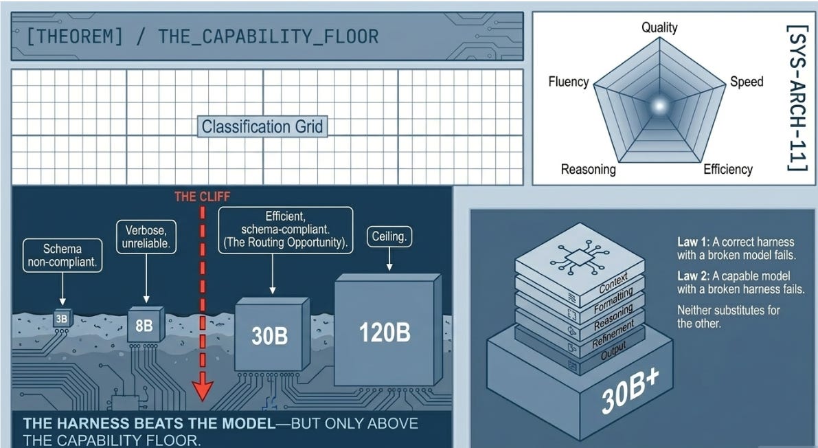
Fix 1 — 8B instead of 3B: E3 improved 30→35/50 but token cost rose 2,327→3,265. The 8B model is more verbose without being capable enough. The finding: for structured analytical generation requiring domain recall and calibrated confidence ratings, 8B is likely insufficient. The minimum viable LIGHT_MODEL for this task is somewhere above 8B — probably 30B+.

Fix 2 — DEFAULT_MODEL probe in E4: Still always task_injected. The probe model was a red herring. The real flaw is gate-prompt misalignment. The gate checks for specific citation names the probe was never given a reason to use. A properly designed E4 gives the probe the minimal anchors first.

Fix 3 — TASK_minimal in E7: Run 1 E7 scored 40/50 at 2,059 tokens. Run 2 E7 scored 25/50 at 4,974 tokens. The context change that helps the 120B model (minimal anchors sufficient) breaks the 8B model (needs full scaffolding). The lesson is the most important single finding across both runs: minimum viable context is model-dependent, not task-dependent.

What Survives: Eight Production-Ready Lessons

Each lesson below is drawn from the Token Tax lab results. Where ASCRS data independently confirms, partially confirms, or contextualises a finding, a note is added inline. The strongest lessons are the ones that appear in both labs unprompted — different task, different scale, same conclusion.

1. Run the compression ablation before building the loop

E1 is the experiment to run first on any new task. Strip context progressively. Find the floor. For frontier-scale models on documented topics, the floor is lower than intuition suggests. For smaller models or niche domains, it will be higher. Knowing the floor changes every downstream architectural decision — you cannot find it without running the ablation. This principle held across both runs without contradiction.

2. Verifier compression is the highest single-lever efficiency gain

E6’s 96% verifier token reduction held across both runs, was consistent across both sessions, and scales with harness complexity. In a V5 harness with a retry loop, the same compact gate applied to every verification step saves orders of magnitude more tokens than any architectural change. Use the full verifier for calibration and auditing. Use the compact gate for production runs once quality is stable.

3. Early exit belongs in every retry loop — unconditionally

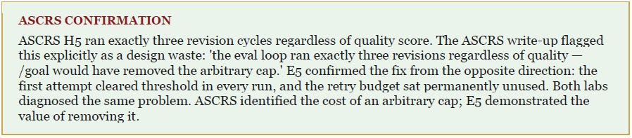
E5 confirmed this in both runs with no exceptions. One conditional check. No downside. In more complex harnesses it saves significant token cost. Add it by default.

4. Schema compression is the lowest-risk efficiency intervention

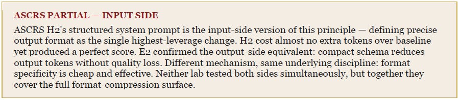
E2 confirmed its prediction exactly in both runs. It changes output format without touching model selection, context injection, or verification logic. Apply it first when efficiency is a concern. Test the counterargument dimension specifically, as that is where compact formats lose nuance most readily.

5. Model routing requires empirical capability validation, not assumptions

E3’s failure across both runs does not invalidate the ASCRS H7 result — it contextualises it. The routing principle is sound. The precondition is knowing the capability floor for your specific task and ensuring LIGHT_MODEL sits above it. Run a test call with your actual system prompt before building the routing layer. Do not assume parameter count predicts task performance.

6. Conditional context needs gate-prompt alignment

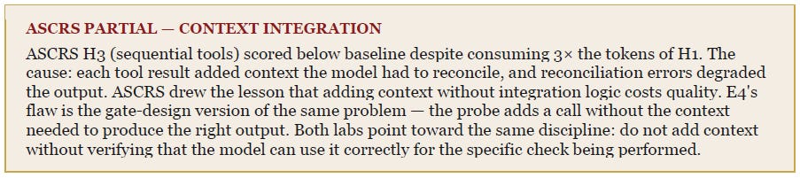
E4’s design flaw was running a fully blind probe and checking for specific citation names the probe had no reason to use. The corrected design gives the probe the minimal anchors and checks for citation fidelity. This maps directly to the Microsoft Azure SRE Agent’s progressive context discovery pattern — check whether the model already has what it needs before providing more.

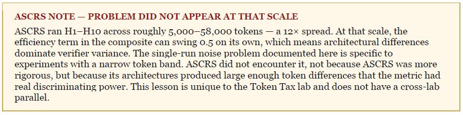
7. Single-run composite rankings are noisy in narrow token bands

If your token range across all configurations is under 10×, run each configuration at least three times and average the results. Single-run rankings in a 2.5× token band are dominated by verifier variance. This is manageable in an experiment and a calibration problem in production. The composite metric is correct in structure; give it stable inputs.

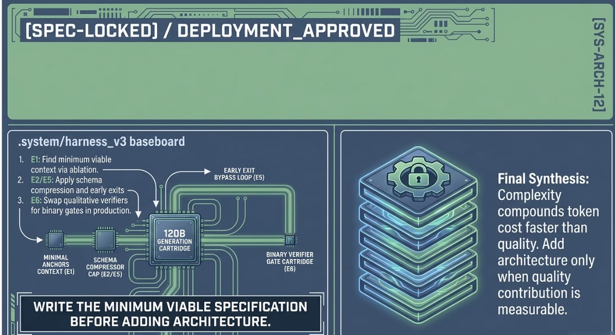
8. Complexity compounds token cost faster than quality

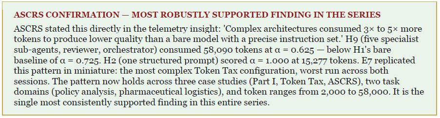
E7 was the most complex configuration in the experiment. It was also the worst result in both sessions. This pattern appeared in the ASCRS lab too — H9 (five-agent swarm) scored below the bare baseline at the highest token cost. The principle is consistent across both labs, both task domains, and both scales: add a new harness layer only when you can measure its quality contribution, and always track its token cost simultaneously. Without tracking, complexity accumulates invisibly.

On the Harness-vs-Model Question

The two runs raise a natural challenge to Part I’s central claim. If changing LIGHT_MODEL from 3B to 8B materially changed E3’s results, does that not suggest the model matters more than the harness? Note: The third run, and Postnote make this more of an issue?

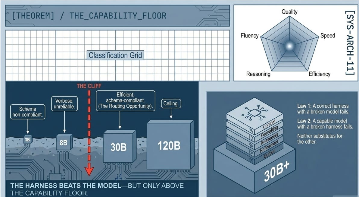
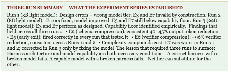
No — but it requires a precise answer. The harness-beats-model principle operates above a capability floor. Below that floor, no harness can compensate for what the model cannot do. The 3B model is not a weaker version of 120B for this task — it is below the threshold where structured analytical reasoning with named evidence is possible at all. Correcting from 3B to 8B is not choosing a better model for performance reasons. It is finding the minimum engine before building the car.

The harness is the primary performance variable for any model above the task’s capability floor. The capability floor is a task-model pair property. Establishing it empirically is the first step in harness design, not an afterthought.

Once above the floor — as the 120B DEFAULT model clearly is in every run — the harness takes over completely. E1_minimal demonstrates this: four study anchors and the same system prompt as baseline produced results indistinguishable from full context injection. The model’s weights held the knowledge. The harness shaped how it was expressed.

The Subscription Economics Argument, Recalibrated

A prior article mentioned that flat-rate AI subscriptions were designed for conversational use but are being consumed by agentic workflows at 5–10× the token rate. That argument stands — but the magnitude demonstrated here is smaller than predicted.

The actual best token saving with quality intact was E2 at 24%, not the predicted 50–60% from E7. Against a V2+V3 baseline of 2,665 tokens, a 24% saving is 639 tokens per task — meaningful, but not transformative. Against a V5 baseline of 7,000 tokens, the same E2 saving (same absolute tokens) plus E6’s verifier compression combined would produce a 35–45% saving. That is where the subscription economics argument bites.

The practical guidance for practitioners running agentic workflows under subscription constraints is: apply the strategies that confirmed cleanly (E2 schema compression, E6 verifier compression, E5 early exit, E1 ablation) against the most expensive harness you are running — which is always the one with the active retry loop and full verification. Not against a lean two-call baseline where the savings have no room to accumulate.

The experiment demonstrated the measurement framework and confirmed three strategies cleanly. It failed to demonstrate the composite winner because the baseline was too lean and one model was too weak. The strategies are right. They need a more complex harness to show their full force.

Thoughts - Based on Two Runs

Two runs of seven experiments produced a result that was more honest than the one predicted. The predicted composite winner (E7) was the actual worst run. The predicted collapse (E1_minimal) never materialised. Three experiments failed for identifiable design reasons. Five produced portable, replicable principles.

That is not a failed experiment. It is an experiment that required two runs to find its actual findings — which is exactly what controlled experiments are supposed to do. The token efficiency strategies confirmed here (schema compression, verifier compression, early exit, context ablation) are real, measurable, and applicable to any production agentic harness above V2+V3 complexity.

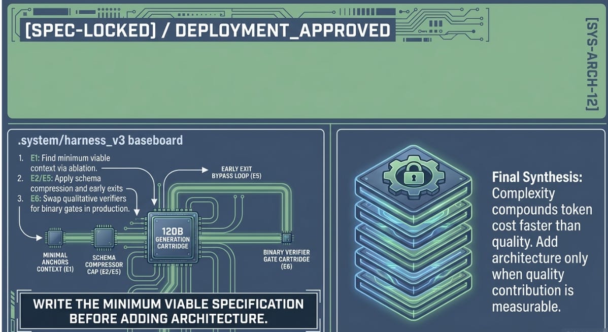
The one that did not need confirming — because it held in every run of every lab documented in this series — is the broadest principle: complexity compounds cost faster than it compounds quality. Measure both. Add layers only when you can justify their cost. The harness is the car. Build it efficiently.

POST NOTE

Run 3 — What a capable light model changed

After Run 2 was complete, a third partial run was conducted — targeting only the two experiments that the light model had broken. The question was simple: if the 8B model was the bottleneck, does replacing it with a +-30B model fix both E3 and E7?

Model change: LIGHT_MODEL changed from meta-llama/llama-3.1-8b-instruct to qwen/qwen3-235b-a22b. Everything else — topic, system prompt, context files, verifier, composite metric — unchanged.

No existing results were modified. Run 3 wrote to an isolated folder with its own results file.

Run 3 Results — E3 and E7

E7 attempt 1 result: Valid output, 40/50, early exit fired immediately. No retry, no collapse. Compare this to Run 2 where attempt 1 returned 0/50 — invalid structured output — forced a retry, and still only recovered to 25/50 on attempt 2 at 4,974 tokens across 4 API calls. Run 3 achieved a better score in 2 API calls at 2,586 tokens.

Full Prediction Scorecard — All Three Runs

The table below consolidates predictions, Run 2 actuals, and Run 3 corrections into a single snapshot. Green = confirmed or exceeded. Amber = contradicted. A dash in the Run 3 column means the experiment was not retested — either it had already confirmed cleanly or its flaw was model-independent.

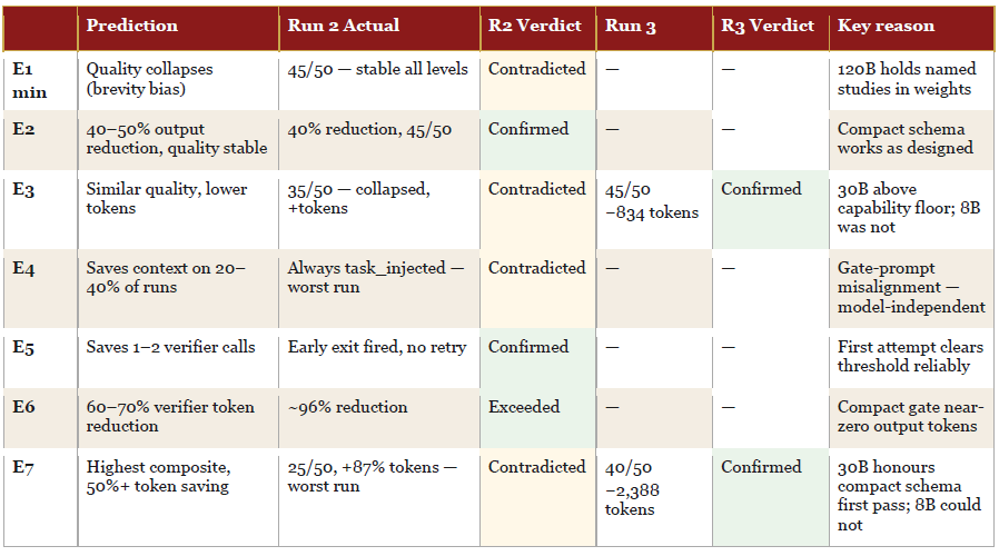
The scorecard tells a cleaner story than the raw results tables. Three predictions were confirmed or exceeded across all runs without model dependency (E2, E5, E6). Two predictions that were contradicted in Run 2 were confirmed in Run 3 once the model was correct (E3, E7). Two remain contradicted because the flaw was in the design, not the model (E1 brevity bias never appeared; E4 gate-prompt misalignment is model-independent). Five of seven predictions are now in the confirmed column across the full experiment series.

The harness design for E7 was correct all along

Run 2’s E7 verdict felt like a failure of architecture — compact schema plus minimal context plus early exit producing the worst result in the lab. Run 3 shows the architecture was never the problem. With a light model capable of honouring the compact schema on a first pass, E7 did exactly what it was designed to do: lowest token cost among multi-call configurations, no wasted retry cycle, score above the quality threshold. The bottleneck in Runs 1 and 2 was the generation model’s capability floor, not the harness design.

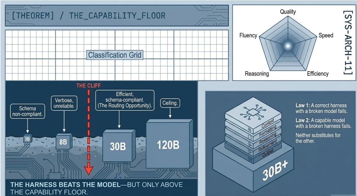
The capability floor for this task sits between 8B and 30B

Three data points now define the curve for structured analytical generation with named evidence and calibrated confidence:

This is not a universal rule. The capability floor is a task-model pair property, as E1 demonstrated from the context side. But for structured analytical generation requiring domain recall, schema compliance, and calibrated reasoning, 30B appears to be the minimum viable routing tier. Below that, the saving on generation cost is outweighed by quality degradation and verbose output that increases token count rather than reducing it.

E3 improved quality and reduced tokens simultaneously

In Runs 1 and 2, E3 was the lab’s worst-efficiency result — quality collapse at higher token cost than baseline. Run 3 reversed both simultaneously: 45/50 at 2,431 tokens is a better quality-per-token ratio than baseline’s 50/50 at 2,665. The model routing principle from ASCRS H7 holds. It required a capable light model to show its effect.

E6 remains the highest single-lever finding

Run 3 did not retest E6 — it was already clean across both prior runs. Its 96% verifier token reduction is independent of light model capability because E6 only touches the verifier side. The two findings that compound best in production are E6 (cut verification cost) and a corrected E7 with a 30B+ light model (cut generation cost without quality loss). Together they represent the most practically applicable output of this entire lab.

References

From This Series

[1] Harness Engineering: A First Principles Build Guide (Part I). Policy brief agent V0–V5, 50/50 final score. Interesting Engineering++, 2026.

[2] ASCRS Harness Lab — The Integrated Agentic Stack. H1–H10 controlled benchmark, May 17, 2026.

Research Papers

[3] Zhang, Q. et al. (2025/2026). Agentic Context Engineering (ACE): Evolving Contexts for Self-Improving Language Models. arXiv:2510.04618. Identifies brevity bias — the tendency for iterative optimisation to collapse toward short, generic prompts that lose critical signal. https://arxiv.org/abs/2510.04618

[4] Liu et al. (2023). AgentBench: Evaluating LLMs as Agents. Stanford/Tsinghua. Source of 6× performance gap finding from harness design alone. https://arxiv.org/abs/2308.03688

[5] Zhu et al. (April 2026). SemaClaw: A Step Towards General-Purpose Personal AI Agents through Harness Engineering. arXiv:2604.11548. https://arxiv.org/abs/2604.11548

[6] Vishnyakova, V. (March 2026). Context Engineering: From Prompts to Corporate Multi-Agent Architecture. arXiv:2603.09619. https://arxiv.org/abs/2603.09619

Production Case Studies & Practitioner Guides

[7] Microsoft Azure SRE Team (April 14, 2026). Harness Engineering for Azure SRE Agent: Building the Agent Self-Improvement Loop. Progressive context discovery pattern. https://techcommunity.microsoft.com/blog/appsonazureblog/the-agent-that-investigates-itself/4500073

[8] Hashimoto, M. (February 5, 2026). My AI Adoption Journey. Origin of harness engineering. Step 5: Engineer the Harness. https://mitchellh.com/writing/my-ai-adoption-journey

[9] Lopopolo, R. / OpenAI (February 11, 2026). Harness Engineering: Leveraging Codex in an Agent-First World. https://openai.com/index/harness-engineering/

[10] Böckeler, B. / Martin Fowler (April 2, 2026). Harness Engineering for Coding Agent Users. https://martinfowler.com/articles/harness-engineering.html

[11] Augment Code (April 17, 2026). Harness Engineering for AI Coding Agents: Constraints That Ship Reliable Code. Hashline experiment: one harness change moved a model from 6.7% to 68.3%. https://www.augmentcode.com/guides/harness-engineering-ai-coding-agents

[12] TechTimes (May 13, 2026). Harness Engineering Emerges as the Fourth Paradigm of AI Engineering. https://www.techtimes.com/articles/316587/20260513/harness-engineering-emerges-fourth-paradigm-ai-engineering.htm

[13] Atlan (April 13, 2026). What Is Harness Engineering AI? The Definitive 2026 Guide. https://atlan.com/know/what-is-harness-engineering/